

196
Elements of Spatial Data Analysis in Ecological Assessments
TABLE 13.5. Landscape metrics: methods, description of characteristics, and factors influencing metric values.
Percent
Aggregation
Frequency
Spatial
System
Landscape
representation
of classes
distribution
distribution
property
Description
metrics
of map classes
into patches
of patch size
of patches
Nonspatial
Composition
Proportion
X
Richness
X
Evenness
X
Dominance
X
Spatial
Configuration
Size
X
X
Shape
X
Edge
X
Perimeter-area ratio
X
X
Density
X
Connectivity
X
X
X
Fractal dimension
X
X
Contagion
X
X
X
X
Source: Hargis et aI., 1997; Gustafson, 1998. See text for further explanation.
variation can then be partitioned into environmental (ENV) and spatial (S) components. By analyzing the overlap between these two components,
variation can be partitioned further into three fractions. Fraction [a] corresponds to the portion ofthe
variation remaining after the spatial structure common to both environmental and spatial explanatory
variables (fraction [b)) has been removed. If [b] is
large, there is support for the hypothesis that the
apparent variable correlations are false; that is,
there is no significant correlation among the variables other than a common spatial structure. Depending on the objectives, there may be interest in
any of the fractions [a], [b], [c], or in U. For example, [c] may be caused by environmental variables that were not included in the analysis or by
historical events or processes that may be masked
by some dominant environmental effect (Borcard
and Legendre, 1994). Analyzing [c] allows the generation of hypotheses about the processes responsible for the observed residual spatial pattern. This
correlative approach is part of ED A (Section 13.2).
Two methods for partitioning variation have been
proposed and widely used: the partial Mantel test
and partial constrained ordinations.
The partial Mantel test (Smouse et aI., 1986; Legendre and Troussellier, 1988) was designed to test
the effect of a geographic variable (i.e., distance)
on two other variables. This test is the multivariate
equivalent of a partial correlation coefficient (Sokal
and Rohlf, 1995). The degree of relationship between two matrices is computed after the effect of
a third matrix has been removed. The question of
whether there is a significant correlation between
the two matrices, other than a common spatial
structure, can then be answered. A drawback is that
the test of significance is conducted on all variables
simultaneously; therefore, determining the specific
source of variation is not possible.
A method to implement the partitioning of variation into specific sources was proposed by Borcard et al. (1992) using partial redundancy analysis (RDA) or canonical analysis of correspondence
(CCA) (ter Braak, 1988; Borcard et aI., 1992; Legendre, 1993; Palmer, 1993). Partial RDA and
CCA quantify the relative contributions of several
categories of variables; randomization tests are
used to assess their significance (ter Braak, 1990).
Specific hypotheses can be tested, further supporting models of causal relationships (Legendre and
Legendre, 1998). Figure 13.2 summarizes some of
the possible interpretations of the various fractions
of variation. These interpretations can help formulate better models for further testing.
13.3.3 Landscape Metrics
In response to the growing demand for measurement and monitoring of regional landscape-level
patterns and processes (e.g., the U.S. Environmental Protection Agency's Environmental Monitoring
and Assessment Program: see Overton et al., 1990;
Hunsaker et aI., 1994), a family of metrics, known
as landscape metrics (Baker and Cai, 1992; Li and
Reynolds, 1995; McGarigal and Marks, 1995; Riitters et aI., 1995; Gustafson, 1998), has recently
been developed to take advantage of the increasing
availability of categorical map data derived from
aerial photographs or satellite images. The geometric and spatial properties of discrete data
mapped into patches (i.e., spatially homogeneous
entities) can be analyzed using two families oflandscape metrics that characterize different properties
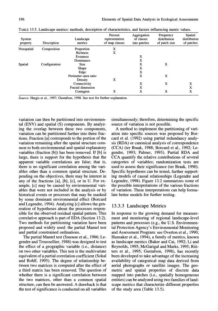
of the study area (Table 13.5).
Elements of Spatial Data Analysis in Ecological Assessments
TABLE 13.5. Landscape metrics: methods, description of characteristics, and factors influencing metric values.
Percent
Aggregation
Frequency
Spatial
System
Landscape
representation
of classes
distribution
distribution
property
Description
metrics
of map classes
into patches
of patch size
of patches
Nonspatial
Composition
Proportion
X
Richness
X
Evenness
X
Dominance
X
Spatial
Configuration
Size
X
X
Shape
X
Edge
X
Perimeter-area ratio
X
X
Density
X
Connectivity
X
X
X
Fractal dimension
X
X
Contagion
X
X
X
X
Source: Hargis et aI., 1997; Gustafson, 1998. See text for further explanation.
variation can then be partitioned into environmental (ENV) and spatial (S) components. By analyzing the overlap between these two components,
variation can be partitioned further into three fractions. Fraction [a] corresponds to the portion ofthe
variation remaining after the spatial structure common to both environmental and spatial explanatory
variables (fraction [b)) has been removed. If [b] is
large, there is support for the hypothesis that the
apparent variable correlations are false; that is,
there is no significant correlation among the variables other than a common spatial structure. Depending on the objectives, there may be interest in
any of the fractions [a], [b], [c], or in U. For example, [c] may be caused by environmental variables that were not included in the analysis or by
historical events or processes that may be masked
by some dominant environmental effect (Borcard
and Legendre, 1994). Analyzing [c] allows the generation of hypotheses about the processes responsible for the observed residual spatial pattern. This
correlative approach is part of ED A (Section 13.2).
Two methods for partitioning variation have been
proposed and widely used: the partial Mantel test
and partial constrained ordinations.
The partial Mantel test (Smouse et aI., 1986; Legendre and Troussellier, 1988) was designed to test
the effect of a geographic variable (i.e., distance)
on two other variables. This test is the multivariate
equivalent of a partial correlation coefficient (Sokal
and Rohlf, 1995). The degree of relationship between two matrices is computed after the effect of
a third matrix has been removed. The question of
whether there is a significant correlation between
the two matrices, other than a common spatial
structure, can then be answered. A drawback is that
the test of significance is conducted on all variables
simultaneously; therefore, determining the specific
source of variation is not possible.
A method to implement the partitioning of variation into specific sources was proposed by Borcard et al. (1992) using partial redundancy analysis (RDA) or canonical analysis of correspondence
(CCA) (ter Braak, 1988; Borcard et aI., 1992; Legendre, 1993; Palmer, 1993). Partial RDA and
CCA quantify the relative contributions of several
categories of variables; randomization tests are
used to assess their significance (ter Braak, 1990).
Specific hypotheses can be tested, further supporting models of causal relationships (Legendre and
Legendre, 1998). Figure 13.2 summarizes some of
the possible interpretations of the various fractions
of variation. These interpretations can help formulate better models for further testing.
13.3.3 Landscape Metrics
In response to the growing demand for measurement and monitoring of regional landscape-level
patterns and processes (e.g., the U.S. Environmental Protection Agency's Environmental Monitoring
and Assessment Program: see Overton et al., 1990;
Hunsaker et aI., 1994), a family of metrics, known
as landscape metrics (Baker and Cai, 1992; Li and
Reynolds, 1995; McGarigal and Marks, 1995; Riitters et aI., 1995; Gustafson, 1998), has recently
been developed to take advantage of the increasing
availability of categorical map data derived from
aerial photographs or satellite images. The geometric and spatial properties of discrete data
mapped into patches (i.e., spatially homogeneous
entities) can be analyzed using two families oflandscape metrics that characterize different properties
of the study area (Table 13.5).