

13.3 Overview of Approaches in Spatial Analysis
195
,
,
,
a
,
b
,
c
,
,
,
,
ENV
I
1
I
t
I
S
I
•
E
· - uFraction
Example of factors that can be used in interpretation
[a]
Nonspatially structured component of biotic or environmental factors
[b]
Spatially structured component of biotic or environmental factors
Spatial autocorrelation in B and ENV
[c]
Spatially structured biotic or environmental factors not included in the analysis
Spatial autocorrelation in B
U
Factors not included in an analysis and nonspatial1y structured at scale of study
Random variation, measurement error
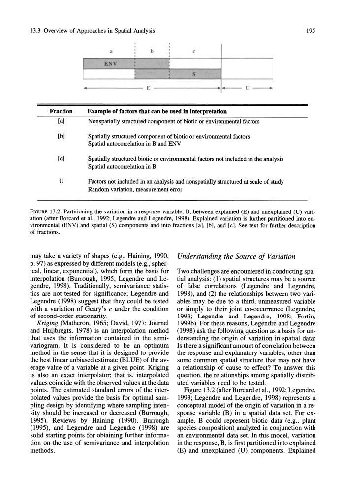
FIGURE 13.2. Partitioning the variation in a response variable, B, between explained (E) and unexplained (U) variation (after Borcard et aI., 1992; Legendre and Legendre, 1998). Explained variation is further partitioned into environmental (ENV) and spatial (S) components and into fractions [a], [b], and [c]. See text for further description
of fractions.
may take a variety of shapes (e.g., Haining, 1990,
p. 97) as expressed by different models (e.g., spherical, linear, exponential), which form the basis for
interpolation (Burrough, 1995; Legendre and Legendre, 1998). Traditionally, semivariance statistics are not tested for significance; Legendre and
Legendre (1998) suggest that they could be tested
with a variation of Geary's c under the condition
of second-order stationarity.
Kriging (Matheron, 1965; David, 1977; 10umel
and Huijbregts, 1978) is an interpolation method
that uses the information contained in the semivariogram. It is considered to be an optimum
method in the sense that it is designed to provide
the best linear unbiased estimate (BLUE) of the average value of a variable at a given point. Kriging
is also an exact interpolator; that is, interpolated
values coincide with the observed values at the data
points. The estimated standard errors of the interpolated values provide the basis for optimal sampling design by identifying where sampling intensity should be increased or decreased (Burrough,
1995). Reviews by Haining (1990), Burrough
(1995), and Legendre and Legendre (1998) are
solid starting points for obtaining further information on the use of semi variance and interpolation
methods.
Understanding the Source of Variation
Two challenges are encountered in conducting spatial analysis: (1) spatial structures may be a source
of false correlations (Legendre and Legendre,
1998), and (2) the relationships between two variables may be due to a third, unmeasured variable
or simply to their joint co-occurrence (Legendre,
1993; Legendre and Legendre, 1998; Fortin,
1999b). For these reasons, Legendre and Legendre
(1998) ask the following question as a basis for understanding the origin of variation in spatial data:
Is there a significant amount of correlation between
the response and explanatory variables, other than
some common spatial structure that may not have
a relationship of cause to effect? To answer this
question, the relationships among spatially distributed variables need to be tested.
Figure 13.2 (after Borcard et al., 1992; Legendre,
1993; Legendre and Legendre, 1998) represents a
conceptual model of the origin of variation in a response variable (B) in a spatial data set. For example, B could represent biotic data (e.g., plant
species composition) analyzed in conjunction with
an environmental data set. In this model, variation
in the response, B, is first partitioned into explained
(E) and unexplained (U) components. Explained
195
,
,
,
a
,
b
,
c
,
,
,
,
ENV
I
1
I
t
I
S
I
•
E
· - uFraction
Example of factors that can be used in interpretation
[a]
Nonspatially structured component of biotic or environmental factors
[b]
Spatially structured component of biotic or environmental factors
Spatial autocorrelation in B and ENV
[c]
Spatially structured biotic or environmental factors not included in the analysis
Spatial autocorrelation in B
U
Factors not included in an analysis and nonspatial1y structured at scale of study
Random variation, measurement error
FIGURE 13.2. Partitioning the variation in a response variable, B, between explained (E) and unexplained (U) variation (after Borcard et aI., 1992; Legendre and Legendre, 1998). Explained variation is further partitioned into environmental (ENV) and spatial (S) components and into fractions [a], [b], and [c]. See text for further description
of fractions.
may take a variety of shapes (e.g., Haining, 1990,
p. 97) as expressed by different models (e.g., spherical, linear, exponential), which form the basis for
interpolation (Burrough, 1995; Legendre and Legendre, 1998). Traditionally, semivariance statistics are not tested for significance; Legendre and
Legendre (1998) suggest that they could be tested
with a variation of Geary's c under the condition
of second-order stationarity.
Kriging (Matheron, 1965; David, 1977; 10umel
and Huijbregts, 1978) is an interpolation method
that uses the information contained in the semivariogram. It is considered to be an optimum
method in the sense that it is designed to provide
the best linear unbiased estimate (BLUE) of the average value of a variable at a given point. Kriging
is also an exact interpolator; that is, interpolated
values coincide with the observed values at the data
points. The estimated standard errors of the interpolated values provide the basis for optimal sampling design by identifying where sampling intensity should be increased or decreased (Burrough,
1995). Reviews by Haining (1990), Burrough
(1995), and Legendre and Legendre (1998) are
solid starting points for obtaining further information on the use of semi variance and interpolation
methods.
Understanding the Source of Variation
Two challenges are encountered in conducting spatial analysis: (1) spatial structures may be a source
of false correlations (Legendre and Legendre,
1998), and (2) the relationships between two variables may be due to a third, unmeasured variable
or simply to their joint co-occurrence (Legendre,
1993; Legendre and Legendre, 1998; Fortin,
1999b). For these reasons, Legendre and Legendre
(1998) ask the following question as a basis for understanding the origin of variation in spatial data:
Is there a significant amount of correlation between
the response and explanatory variables, other than
some common spatial structure that may not have
a relationship of cause to effect? To answer this
question, the relationships among spatially distributed variables need to be tested.
Figure 13.2 (after Borcard et al., 1992; Legendre,
1993; Legendre and Legendre, 1998) represents a
conceptual model of the origin of variation in a response variable (B) in a spatial data set. For example, B could represent biotic data (e.g., plant
species composition) analyzed in conjunction with
an environmental data set. In this model, variation
in the response, B, is first partitioned into explained
(E) and unexplained (U) components. Explained