

190
Elements of Spatial Data Analysis in Ecological Assessments
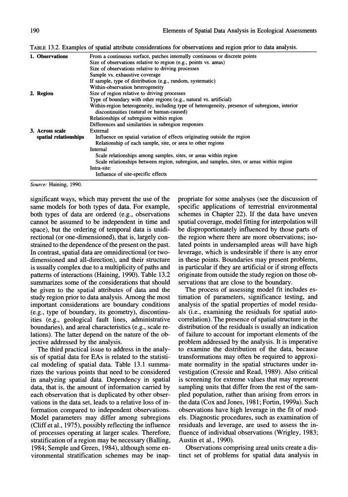
TABLE 13.2. Examples of spatial attribute considerations for observations and region prior to data analysis.
1. Observations
From a continuous surface, patches internally continuous or discrete points
Size of observations relative to region (e.g., points vs. areas)
Size of observations relative to driving processes
Sample vs. exhaustive coverage
If sample, type of distribution (e.g., random, systematic)
Within-observation heterogeneity
2. Region
Size of region relative to driving processes
Type of boundary with other regions (e.g., natural vs. artificial)
Within-region heterogeneity, including type of heterogeneity, presence of subregions, interior
3. Across scale
discontinuities (natural or human-caused)
Relationships of subregions within region
Differences and similarities in SUbregion responses
External
spatial relationsblps
Influence on spatial variation of effects originating outside the region
Relationship of each sample, site, or area to other regions
Internal
Scale relationships among samples, sites, or areas within region
Scale relationships between region, subregion, and samples, sites, or areas within region
Intra-site:
Influence of site-specific effects
Source: Haining, 1990.
significant ways, which may prevent the use of the
same models for both types of data. For example,
both types of data are ordered (e.g., observations
cannot be assumed to be independent in time and
space), but the ordering of temporal data is unidirectional (or one-dimensioned), that is, largely constrained to the dependence of the present on the past.
In contrast, spatial data are omnidirectional (or twodimensioned and all-direction), and their structure
is usually complex due to a multiplicity of paths and
patterns of interactions (Haining, 1990). Table 13.2
summarizes some of the considerations that should
be given to the spatial attributes of data and the
study region prior to data analysis. Among the most
important considerations are boundary conditions
(e.g., type of boundary, its geometry), discontinuities (e.g., geological fault lines, administrative
boundaries), and areal characteristics (e.g., scale relations). The latter depend on the nature of the objective addressed by the analysis.
The third practical issue to address in the analysis of spatial data for EAs is related to the statistical modeling of spatial data. Table 13.1 summarizes the various points that need to be considered
in analyzing spatial data. Dependency in spatial
data, that is, the amount of information carried by
each observation that is duplicated by other observations in the data set, leads to a relative loss of information compared to independent observations.
Model parameters may differ among subregions
(Cliff et al., 1975), possibly reflecting the influence
of processes operating at larger scales. Therefore,
stratification of a region may be necessary (Balling,
1984; Semple and Green, 1984), although some environmental stratification schemes may be inappropriate for some analyses (see the discussion of
specific applications of terrestrial environmental
schemes in Chapter 22). If the data have uneven
spatial coverage, model fitting for interpolation will
be disproportionately influenced by those parts of
the region where there are more observations; isolated points in undersampled areas will have high
leverage, which is undesirable if there is any error
in these points. Boundaries may present problems,
in particular if they are artificial or if strong effects
originate from outside the study region on those observations that are close to the boundary.
The process of assessing model fit includes estimation of parameters, significance testing, and
analysis of the' spatial properties of model residuals (i.e., examining the residuals for spatial autocorrelation). The presence of spatial structure in the
distribution of the residuals is usually an indication
of failure to account for important elements of the
problem addressed by the analysis. It is imperative
to examine the distribution of the data, because
transformations may often be required to approximate normality in the spatial structures under investigation (Cressie and Read, 1989). Also critical
is screening for extreme values that may represent
sampling units that differ from the rest of the sampled population, rather than arising from errors in
the data (Cox and Jones, 1981; Fortin, 1999a). Such
observations have high leverage in the fit of models. Diagnostic procedures, such as examination of
residuals and leverage, are used to assess the influence of individual observations (Wrigley, 1983;
Austin et al., 1990).
Observations comprising areal units create a distinct set of problems for spatial data analysis in
Elements of Spatial Data Analysis in Ecological Assessments
TABLE 13.2. Examples of spatial attribute considerations for observations and region prior to data analysis.
1. Observations
From a continuous surface, patches internally continuous or discrete points
Size of observations relative to region (e.g., points vs. areas)
Size of observations relative to driving processes
Sample vs. exhaustive coverage
If sample, type of distribution (e.g., random, systematic)
Within-observation heterogeneity
2. Region
Size of region relative to driving processes
Type of boundary with other regions (e.g., natural vs. artificial)
Within-region heterogeneity, including type of heterogeneity, presence of subregions, interior
3. Across scale
discontinuities (natural or human-caused)
Relationships of subregions within region
Differences and similarities in SUbregion responses
External
spatial relationsblps
Influence on spatial variation of effects originating outside the region
Relationship of each sample, site, or area to other regions
Internal
Scale relationships among samples, sites, or areas within region
Scale relationships between region, subregion, and samples, sites, or areas within region
Intra-site:
Influence of site-specific effects
Source: Haining, 1990.
significant ways, which may prevent the use of the
same models for both types of data. For example,
both types of data are ordered (e.g., observations
cannot be assumed to be independent in time and
space), but the ordering of temporal data is unidirectional (or one-dimensioned), that is, largely constrained to the dependence of the present on the past.
In contrast, spatial data are omnidirectional (or twodimensioned and all-direction), and their structure
is usually complex due to a multiplicity of paths and
patterns of interactions (Haining, 1990). Table 13.2
summarizes some of the considerations that should
be given to the spatial attributes of data and the
study region prior to data analysis. Among the most
important considerations are boundary conditions
(e.g., type of boundary, its geometry), discontinuities (e.g., geological fault lines, administrative
boundaries), and areal characteristics (e.g., scale relations). The latter depend on the nature of the objective addressed by the analysis.
The third practical issue to address in the analysis of spatial data for EAs is related to the statistical modeling of spatial data. Table 13.1 summarizes the various points that need to be considered
in analyzing spatial data. Dependency in spatial
data, that is, the amount of information carried by
each observation that is duplicated by other observations in the data set, leads to a relative loss of information compared to independent observations.
Model parameters may differ among subregions
(Cliff et al., 1975), possibly reflecting the influence
of processes operating at larger scales. Therefore,
stratification of a region may be necessary (Balling,
1984; Semple and Green, 1984), although some environmental stratification schemes may be inappropriate for some analyses (see the discussion of
specific applications of terrestrial environmental
schemes in Chapter 22). If the data have uneven
spatial coverage, model fitting for interpolation will
be disproportionately influenced by those parts of
the region where there are more observations; isolated points in undersampled areas will have high
leverage, which is undesirable if there is any error
in these points. Boundaries may present problems,
in particular if they are artificial or if strong effects
originate from outside the study region on those observations that are close to the boundary.
The process of assessing model fit includes estimation of parameters, significance testing, and
analysis of the' spatial properties of model residuals (i.e., examining the residuals for spatial autocorrelation). The presence of spatial structure in the
distribution of the residuals is usually an indication
of failure to account for important elements of the
problem addressed by the analysis. It is imperative
to examine the distribution of the data, because
transformations may often be required to approximate normality in the spatial structures under investigation (Cressie and Read, 1989). Also critical
is screening for extreme values that may represent
sampling units that differ from the rest of the sampled population, rather than arising from errors in
the data (Cox and Jones, 1981; Fortin, 1999a). Such
observations have high leverage in the fit of models. Diagnostic procedures, such as examination of
residuals and leverage, are used to assess the influence of individual observations (Wrigley, 1983;
Austin et al., 1990).
Observations comprising areal units create a distinct set of problems for spatial data analysis in