

where p(x,j|i) is the probability that an individual leaving from a point
chosen in patch i lands on a point in patch j after traveling a distance x
and p(m) is the probability that migration occurs at all. To get from
the conditional probability p(j|i) to the probability of a transition from
i to j, we must estimate the probability that the individual started in
patch i. Then, p(i,j) = p(i)p(j|i), where p(i) is the probability the individual
was found in patch i.
The matrix of probabilities A with elements a ij = p(i,j) defines a landscape
network. The network can be thought of as a graph (Harary 1969; Urban
and Keitt 2001) in which each patch is a graph “node” and connections
between patches are represented as graph “edges.” We can assign distances
to these edges, either as true distances between patches or as a “functional
distance” related to transition probabilities between patches. A convenient
measure of the functional distance is d ij = 1/a ij (i.e., the mean time between
immigration from i to j).
Estimation of p ij can be accomplished in a number of ways. The dispersal function p(x) and the migration probability p m can be estimated by
tracking animal movements (telemetry) or by mark-recapture methods.
Once p(x) is estimated, the patch transition probabilities p(i,j) can then
be estimated on the basis of a habitat map that provides the estimates
of p(x,j|i). For more complex dispersal behavior, migration rates can be
estimated directly through simulation modeling of the migration process.
The important point is that landscape network models directly incorporate
actual patterns of habitat fragmentation into the model structure, as
opposed to approaches that assume space is uniform [Hanski and
Simberloff (1997) refer to these as “spatially realistic models”]. Thus, landscape network analysis is a powerful tool for analyzing real landscapes and
can be used as a basis for building more complex population viability
models.
As specified, the landscape network connected every patch to every other
patch, albeit sometimes with very low probability. The dense network of
connections makes graphical interpretation of the network difficult. A
feature that is much simpler to analyze is the spanning tree of a network.
A “tree” is simply a graph with no loops, and a spanning tree is a tree that
contains all nodes (patches) in the network. In particular, the minimumlength spanning tree (MST) is an interesting feature of the network because
it identifies the “backbone” or connected core of the landscape. The
minimum spanning tree is the spanning tree that has the shortest total
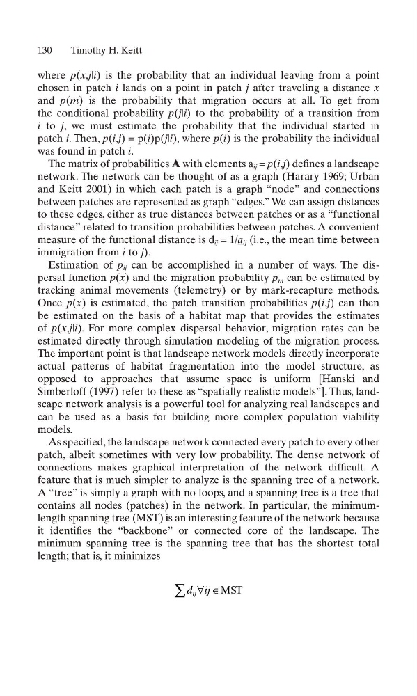
length; that is, it minimizes
d ij
ij ∀ ∈
∑
MST
130
Timothy H. Keitt
chosen in patch i lands on a point in patch j after traveling a distance x
and p(m) is the probability that migration occurs at all. To get from
the conditional probability p(j|i) to the probability of a transition from
i to j, we must estimate the probability that the individual started in
patch i. Then, p(i,j) = p(i)p(j|i), where p(i) is the probability the individual
was found in patch i.
The matrix of probabilities A with elements a ij = p(i,j) defines a landscape
network. The network can be thought of as a graph (Harary 1969; Urban
and Keitt 2001) in which each patch is a graph “node” and connections
between patches are represented as graph “edges.” We can assign distances
to these edges, either as true distances between patches or as a “functional
distance” related to transition probabilities between patches. A convenient
measure of the functional distance is d ij = 1/a ij (i.e., the mean time between
immigration from i to j).
Estimation of p ij can be accomplished in a number of ways. The dispersal function p(x) and the migration probability p m can be estimated by
tracking animal movements (telemetry) or by mark-recapture methods.
Once p(x) is estimated, the patch transition probabilities p(i,j) can then
be estimated on the basis of a habitat map that provides the estimates
of p(x,j|i). For more complex dispersal behavior, migration rates can be
estimated directly through simulation modeling of the migration process.
The important point is that landscape network models directly incorporate
actual patterns of habitat fragmentation into the model structure, as
opposed to approaches that assume space is uniform [Hanski and
Simberloff (1997) refer to these as “spatially realistic models”]. Thus, landscape network analysis is a powerful tool for analyzing real landscapes and
can be used as a basis for building more complex population viability
models.
As specified, the landscape network connected every patch to every other
patch, albeit sometimes with very low probability. The dense network of
connections makes graphical interpretation of the network difficult. A
feature that is much simpler to analyze is the spanning tree of a network.
A “tree” is simply a graph with no loops, and a spanning tree is a tree that
contains all nodes (patches) in the network. In particular, the minimumlength spanning tree (MST) is an interesting feature of the network because
it identifies the “backbone” or connected core of the landscape. The
minimum spanning tree is the spanning tree that has the shortest total
length; that is, it minimizes
d ij
ij ∀ ∈
∑
MST
130
Timothy H. Keitt