

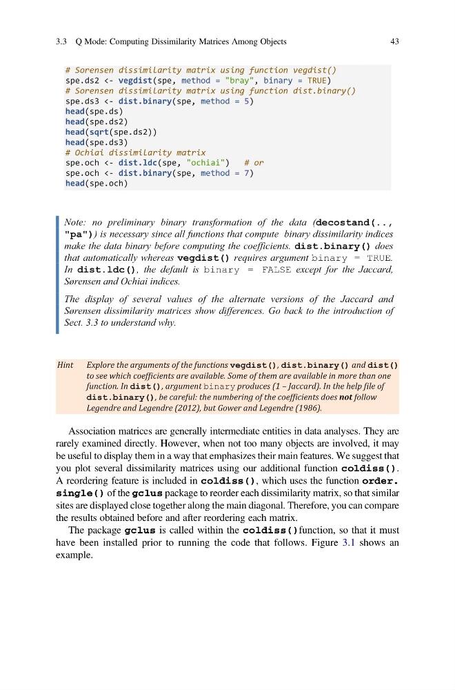
# Sorensen dissimilarity matrix using function vegdist()
spe.ds2 <- vegdist(spe, method = "bray", binary = TRUE)
# Sorensen dissimilarity matrix using function dist.binary()
spe.ds3 <- dist.binary(spe, method = 5)
head(spe.ds)
head(spe.ds2)
head(sqrt(spe.ds2))
head(spe.ds3)
# Ochiai dissimilarity matrix
spe.och <- dist.ldc(spe, "ochiai")
# or
spe.och <- dist.binary(spe, method = 7)
head(spe.och)
Note: no preliminary binary transformation of the data (decostand(..,
"pa")) is necessary since all functions that compute binary dissimilarity indices
make the data binary before computing the coefficients. dist.binary() does
that automatically whereas vegdist() requires argument binary = TRUE.
In dist.ldc(), the default is binary = FALSE except for the Jaccard,
Sørensen and Ochiai indices.
The display of several values of the alternate versions of the Jaccard and
Sørensen dissimilarity matrices show differences. Go back to the introduction of
Sect. 3.3 to understand why.
Hint
Explore the arguments of the functions vegdist(), dist.binary() and dist()
to see which coefϔicients are available. Some of them are available in more than one
function. In dist(), argument binary produces (1 – Jaccard). In the help ϔile of
dist.binary(), be careful: the numbering of the coefϔicients does not follow
Legendre and Legendre (2012), but Gower and Legendre (1986).
Association matrices are generally intermediate entities in data analyses. They are
rarely examined directly. However, when not too many objects are involved, it may
be useful to display them in a way that emphasizes their main features. We suggest that
you plot several dissimilarity matrices using our additional function coldiss().
A reordering feature is included in coldiss(), which uses the function order.
single() of the gclus package to reorder each dissimilarity matrix, so that similar
sites are displayed close together along the main diagonal. Therefore, you can compare
the results obtained before and after reordering each matrix.
The package gclus is called within the coldiss()function, so that it must
have been installed prior to running the code that follows. Figure 3.1 shows an
example.
3.3 Q Mode: Computing Dissimilarity Matrices Among Objects
43
spe.ds2 <- vegdist(spe, method = "bray", binary = TRUE)
# Sorensen dissimilarity matrix using function dist.binary()
spe.ds3 <- dist.binary(spe, method = 5)
head(spe.ds)
head(spe.ds2)
head(sqrt(spe.ds2))
head(spe.ds3)
# Ochiai dissimilarity matrix
spe.och <- dist.ldc(spe, "ochiai")
# or
spe.och <- dist.binary(spe, method = 7)
head(spe.och)
Note: no preliminary binary transformation of the data (decostand(..,
"pa")) is necessary since all functions that compute binary dissimilarity indices
make the data binary before computing the coefficients. dist.binary() does
that automatically whereas vegdist() requires argument binary = TRUE.
In dist.ldc(), the default is binary = FALSE except for the Jaccard,
Sørensen and Ochiai indices.
The display of several values of the alternate versions of the Jaccard and
Sørensen dissimilarity matrices show differences. Go back to the introduction of
Sect. 3.3 to understand why.
Hint
Explore the arguments of the functions vegdist(), dist.binary() and dist()
to see which coefϔicients are available. Some of them are available in more than one
function. In dist(), argument binary produces (1 – Jaccard). In the help ϔile of
dist.binary(), be careful: the numbering of the coefϔicients does not follow
Legendre and Legendre (2012), but Gower and Legendre (1986).
Association matrices are generally intermediate entities in data analyses. They are
rarely examined directly. However, when not too many objects are involved, it may
be useful to display them in a way that emphasizes their main features. We suggest that
you plot several dissimilarity matrices using our additional function coldiss().
A reordering feature is included in coldiss(), which uses the function order.
single() of the gclus package to reorder each dissimilarity matrix, so that similar
sites are displayed close together along the main diagonal. Therefore, you can compare
the results obtained before and after reordering each matrix.
The package gclus is called within the coldiss()function, so that it must
have been installed prior to running the code that follows. Figure 3.1 shows an
example.
3.3 Q Mode: Computing Dissimilarity Matrices Among Objects
43