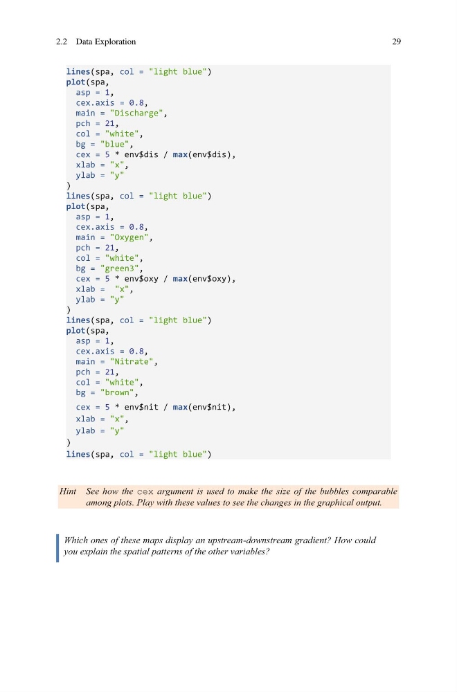
lines(spa, col = "light blue")
plot(spa,
asp = 1,
cex.axis = 0.8,
main = "Discharge",
pch = 21,
col = "white",
bg = "blue",
cex = 5 * env$dis / max(env$dis),
xlab = "x",
ylab = "y"
)
lines(spa, col = "light blue")
plot(spa,
asp = 1,
cex.axis = 0.8,
main = "Oxygen",
pch = 21,
col = "white",
bg = "green3",
cex = 5 * env$oxy / max(env$oxy),
xlab = "x",
ylab = "y"
)
lines(spa, col = "light blue")
plot(spa,
asp = 1,
cex.axis = 0.8,
main = "Nitrate",
pch = 21,
col = "white",
bg = "brown",
cex = 5 * env$nit / max(env$nit),
xlab = "x",
ylab = "y"
)
lines(spa, col = "light blue")
Hint See how the cex argument is used to make the size of the bubbles comparable
among plots. Play with these values to see the changes in the graphical output.
Which ones of these maps display an upstream-downstream gradient? How could
you explain the spatial patterns of the other variables?
2.2 Data Exploration
29