

2.2.5 Environmental Data
Now that we are acquainted with the species data, let us turn to the environmental
data file (object env).
First, go back to Sect. 2.2 and apply the basic functions presented there to the
object env. While examining the summary(), note how the variables differ from
the species data in values and spatial distributions.
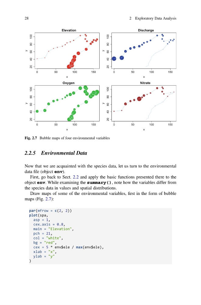
Draw maps of some of the environmental variables, first in the form of bubble
maps (Fig. 2.7):
par(mfrow = c(2, 2))
plot(spa,
asp = 1,
cex.axis = 0.8,
main = "Elevation",
pch = 21,
col = "white",
bg = "red",
cex = 5 * env$ele / max(env$ele),
xlab = "x",
ylab = "y"
)
0
50
100
150
20
40
60
80 100
Elevation
x
y
0
50
100
150
20
40
60
80 100
Discharge
x
y
0
50
100
150
20
40
60
80 100
Oxygen
x
y
0
50
100
150
20
40
60
80 100
Nitrate
x
y
Fig. 2.7 Bubble maps of four environmental variables
28
2 Exploratory Data Analysis
Now that we are acquainted with the species data, let us turn to the environmental
data file (object env).
First, go back to Sect. 2.2 and apply the basic functions presented there to the
object env. While examining the summary(), note how the variables differ from
the species data in values and spatial distributions.
Draw maps of some of the environmental variables, first in the form of bubble
maps (Fig. 2.7):
par(mfrow = c(2, 2))
plot(spa,
asp = 1,
cex.axis = 0.8,
main = "Elevation",
pch = 21,
col = "white",
bg = "red",
cex = 5 * env$ele / max(env$ele),
xlab = "x",
ylab = "y"
)
0
50
100
150
20
40
60
80 100
Elevation
x
y
0
50
100
150
20
40
60
80 100
Discharge
x
y
0
50
100
150
20
40
60
80 100
Oxygen
x
y
0
50
100
150
20
40
60
80 100
Nitrate
x
y
Fig. 2.7 Bubble maps of four environmental variables
28
2 Exploratory Data Analysis