

their spatial distributions are destroyed. Alpha diversity is destroyed as well in the
permutations.
Legendre and De Cáceres (2013) also showed how to calculate LCBD indices
from a dissimilarity matrix. The computation involves the same transformation of
the dissimilarity matrix as the one used in PCoA.
8.4.2.5 Species Contributions to Beta Diversity (SCBD)
Decomposition of beta diversity into species contributions can only be computed
from a site-by-species data table, not from a dissimilarity matrix since the species
abundances at the sites have been lost in the calculation of the dissimilarities.
The contribution of species j to the overall beta diversity is the sum (SS j ) of the
centred and squared values for species (or column) j in matrix S:
SS j ¼
X n
i¼1
s ij
ð8:16Þ
Again, SS Total ¼
X n
i¼1
ss i (Eq. 8.10).
The relative contribution of species j to beta diversity, called the species contribution to beta diversity (SCBD), is:
SCBD j ¼ SS j =SS Total
ð8:17Þ
8.4.2.6 Computation of LCBD and SCBD using beta.div()
of Package adespatial
Legendre and De Cáceres (2013) wrote function beta.div() to compute beta
diversity as Var(Y) and its decomposition into LCBD and SCBD. This function is
now part of the adespatial package. Let us apply it to the Doubs fish data, as the
authors did in their paper, but here we will use the Hellinger instead of the chord
transformation, which is also appropriate. Legendre and De Cáceres (2013) have
shown that the LCBD indices computed from the 11 dissimilarity coefficients
suitable for beta diversity assessment were highly concordant.
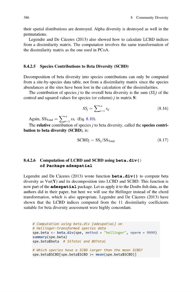
# Computation using beta.div {adespatial} on
# Hellinger-transformed species data
spe.beta <- beta.div(spe, method = "hellinger", nperm = 9999)
summary(spe.beta)
spe.beta$beta # SSTotal and BDTotal
# Which species have a SCBD larger than the mean SCBD?
spe.beta$SCBD[spe.beta$SCBD >= mean(spe.beta$SCBD)]
386
8 Community Diversity
permutations.
Legendre and De Cáceres (2013) also showed how to calculate LCBD indices
from a dissimilarity matrix. The computation involves the same transformation of
the dissimilarity matrix as the one used in PCoA.
8.4.2.5 Species Contributions to Beta Diversity (SCBD)
Decomposition of beta diversity into species contributions can only be computed
from a site-by-species data table, not from a dissimilarity matrix since the species
abundances at the sites have been lost in the calculation of the dissimilarities.
The contribution of species j to the overall beta diversity is the sum (SS j ) of the
centred and squared values for species (or column) j in matrix S:
SS j ¼
X n
i¼1
s ij
ð8:16Þ
Again, SS Total ¼
X n
i¼1
ss i (Eq. 8.10).
The relative contribution of species j to beta diversity, called the species contribution to beta diversity (SCBD), is:
SCBD j ¼ SS j =SS Total
ð8:17Þ
8.4.2.6 Computation of LCBD and SCBD using beta.div()
of Package adespatial
Legendre and De Cáceres (2013) wrote function beta.div() to compute beta
diversity as Var(Y) and its decomposition into LCBD and SCBD. This function is
now part of the adespatial package. Let us apply it to the Doubs fish data, as the
authors did in their paper, but here we will use the Hellinger instead of the chord
transformation, which is also appropriate. Legendre and De Cáceres (2013) have
shown that the LCBD indices computed from the 11 dissimilarity coefficients
suitable for beta diversity assessment were highly concordant.
# Computation using beta.div {adespatial} on
# Hellinger-transformed species data
spe.beta <- beta.div(spe, method = "hellinger", nperm = 9999)
summary(spe.beta)
spe.beta$beta # SSTotal and BDTotal
# Which species have a SCBD larger than the mean SCBD?
spe.beta$SCBD[spe.beta$SCBD >= mean(spe.beta$SCBD)]
386
8 Community Diversity