

proposes one approach to the concept, linked to the variance of the site-by-species
table and to many of the analyses described in this book, which analyse or partition
that variance in different manners.
Beta diversity has been defined in various ways. Whittaker’s (1960) definition is
the variation in species composition among sites within a geographic area of interest.
Different equations exist to measure that variation. From the research on beta
diversity two approaches emerge: (1) Beta diversity can be construed as turnover,
i.e., the directional change in community composition along a predefined spatial,
temporal or environmental gradient. (2) Beta diversity can also be defined as the
variation in community composition among sampling units, without reference to an
explicit gradient. Both concepts are within the scope of Whittaker’s definition.
Many papers have proposed indices of diversity at the three levels. Most of the
proposed measurements of beta diversity are linked to alpha and gamma. In the
multiplicative and additive approaches mentioned in Sect. 8.4.1, beta diversity is a
derived quantity, i.e. it is linked to, and can be obtained only from the measurement
of alpha and gamma. In his introduction to the Forum section in Ecology (2010:
1962–1992), Ellison (2010) called for a measure of beta diversity that would be
computationally independent from the two other levels. Legendre and De Cáceres’
(2013) method fulfils this wish. It uses the total variance of the site-by-species
Table Y, Var(Y), as an estimate of beta diversity, in the line of Pélissier et al.
(2003), Legendre et al. (2005) and Anderson et al. (2006). Var(Y) is calculated
independently from alpha and gamma diversity. Note that the simple ordination
methods presented in Chap. 5 and the constrained ordination methods of Chap. 6 can
be applied to community composition data and be used to analyse and interpret the
patterns of variation of the community composition among sites. Likewise, the
methods of spatial eigenfunction analysis described in Chap. 7 have been developed
to decompose the spatial variation of community data among spatial scales. Therefore, all these methods can be seen as methods of analysis of beta diversity.
8.4.2.2 Computing Beta Diversity as Var(Y)
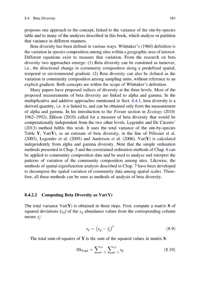
The total variance Var(Y) is obtained in three steps. First, compute a matrix S of
squared deviations [s ij ] of the y ij abundance values from the corresponding column
means
y j :
s ij ¼
À
y ij À
y j
Á 2
ð8:9Þ
The total sum-of-squares of Y is the sum of the squared values in matrix S:
SS Total ¼
X n
i¼1
X p
j¼1
s ij
ð8:10Þ
8.4 Beta Diversity
383
table and to many of the analyses described in this book, which analyse or partition
that variance in different manners.
Beta diversity has been defined in various ways. Whittaker’s (1960) definition is
the variation in species composition among sites within a geographic area of interest.
Different equations exist to measure that variation. From the research on beta
diversity two approaches emerge: (1) Beta diversity can be construed as turnover,
i.e., the directional change in community composition along a predefined spatial,
temporal or environmental gradient. (2) Beta diversity can also be defined as the
variation in community composition among sampling units, without reference to an
explicit gradient. Both concepts are within the scope of Whittaker’s definition.
Many papers have proposed indices of diversity at the three levels. Most of the
proposed measurements of beta diversity are linked to alpha and gamma. In the
multiplicative and additive approaches mentioned in Sect. 8.4.1, beta diversity is a
derived quantity, i.e. it is linked to, and can be obtained only from the measurement
of alpha and gamma. In his introduction to the Forum section in Ecology (2010:
1962–1992), Ellison (2010) called for a measure of beta diversity that would be
computationally independent from the two other levels. Legendre and De Cáceres’
(2013) method fulfils this wish. It uses the total variance of the site-by-species
Table Y, Var(Y), as an estimate of beta diversity, in the line of Pélissier et al.
(2003), Legendre et al. (2005) and Anderson et al. (2006). Var(Y) is calculated
independently from alpha and gamma diversity. Note that the simple ordination
methods presented in Chap. 5 and the constrained ordination methods of Chap. 6 can
be applied to community composition data and be used to analyse and interpret the
patterns of variation of the community composition among sites. Likewise, the
methods of spatial eigenfunction analysis described in Chap. 7 have been developed
to decompose the spatial variation of community data among spatial scales. Therefore, all these methods can be seen as methods of analysis of beta diversity.
8.4.2.2 Computing Beta Diversity as Var(Y)
The total variance Var(Y) is obtained in three steps. First, compute a matrix S of
squared deviations [s ij ] of the y ij abundance values from the corresponding column
means
y j :
s ij ¼
À
y ij À
y j
Á 2
ð8:9Þ
The total sum-of-squares of Y is the sum of the squared values in matrix S:
SS Total ¼
X n
i¼1
X p
j¼1
s ij
ð8:10Þ
8.4 Beta Diversity
383