

=======================================================
Space-time ANOVA without replicates
Pierre Legendre, Miquel De Caceres, Daniel Borcard
=======================================================
Number of space points (s) = 22
Number of time points (tt) = 10
Number of observations (n = s*tt) = 220
Number of response variables (p) = 56
Computing dbMEMs to code for space
Truncation level for space dbMEMs = 1
Computing dbMEMs to code for time
Truncation level for time dbMEMs = 1
Number of space coding functions = 10
Number of time coding functions = 4
MODEL V: HELMERT CONTRAST FOR TESTING MAIN FACTORS.
SPACE AND TIME dbMEMs FOR TESTING INTERACTION.
Number of space variables = 21
Number of time variables = 9
Number of interaction variables = 40
Number of residual degrees of freedom = 149
Interaction test:
R2 = 0.1835
F = 2.313
P( 999 perm) = 0.001
Space test:
R2 = 0.2522
F = 6.0569
P( 999 perm) = 0.001
Time test:
R2 = 0.2688
F = 15.0608
P( 999 perm) = 0.001
------------------------------------------------------Time for this computation = 2.899000 sec
=======================================================
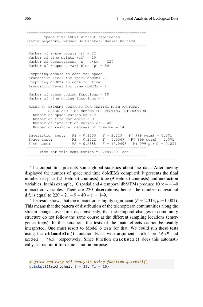
The output first presents some global statistics about the data. After having
displayed the number of space and time dbMEMs computed, it presents the final
number of space (21 Helmert contrasts), time (9 Helmert contrasts) and interaction
variables. In this example, 10 spatial and 4 temporal dbMEMs produce 10 Â 4 ¼ 40
interaction variables. There are 220 observations; hence, the number of residual
d.f. is equal to 220 – 21 – 9 – 40 – 1 ¼ 149.
The result shows that the interaction is highly significant (F ¼ 2.313, p ¼ 0.001).
This means that the pattern of distribution of the trichopteran communities along the
stream changes over time or, conversely, that the temporal changes in community
structure do not follow the same course at the different sampling locations (emergence traps). In this situation, the tests of the main effects cannot be readily
interpreted. One must resort to Model 6 tests for that. We could run these tests
using the stimodels() function twice with argument model ¼ "6a" and
model ¼ "6b" respectively. Since function quicksti() does this automatically, let us run it for demonstration purpose.
# Quick and easy sti analysis using function quicksti()
quicksti(tricho.hel, S = 22, Ti = 10)
366
7 Spatial Analysis of Ecological Data
Space-time ANOVA without replicates
Pierre Legendre, Miquel De Caceres, Daniel Borcard
=======================================================
Number of space points (s) = 22
Number of time points (tt) = 10
Number of observations (n = s*tt) = 220
Number of response variables (p) = 56
Computing dbMEMs to code for space
Truncation level for space dbMEMs = 1
Computing dbMEMs to code for time
Truncation level for time dbMEMs = 1
Number of space coding functions = 10
Number of time coding functions = 4
MODEL V: HELMERT CONTRAST FOR TESTING MAIN FACTORS.
SPACE AND TIME dbMEMs FOR TESTING INTERACTION.
Number of space variables = 21
Number of time variables = 9
Number of interaction variables = 40
Number of residual degrees of freedom = 149
Interaction test:
R2 = 0.1835
F = 2.313
P( 999 perm) = 0.001
Space test:
R2 = 0.2522
F = 6.0569
P( 999 perm) = 0.001
Time test:
R2 = 0.2688
F = 15.0608
P( 999 perm) = 0.001
------------------------------------------------------Time for this computation = 2.899000 sec
=======================================================
The output first presents some global statistics about the data. After having
displayed the number of space and time dbMEMs computed, it presents the final
number of space (21 Helmert contrasts), time (9 Helmert contrasts) and interaction
variables. In this example, 10 spatial and 4 temporal dbMEMs produce 10 Â 4 ¼ 40
interaction variables. There are 220 observations; hence, the number of residual
d.f. is equal to 220 – 21 – 9 – 40 – 1 ¼ 149.
The result shows that the interaction is highly significant (F ¼ 2.313, p ¼ 0.001).
This means that the pattern of distribution of the trichopteran communities along the
stream changes over time or, conversely, that the temporal changes in community
structure do not follow the same course at the different sampling locations (emergence traps). In this situation, the tests of the main effects cannot be readily
interpreted. One must resort to Model 6 tests for that. We could run these tests
using the stimodels() function twice with argument model ¼ "6a" and
model ¼ "6b" respectively. Since function quicksti() does this automatically, let us run it for demonstration purpose.
# Quick and easy sti analysis using function quicksti()
quicksti(tricho.hel, S = 22, Ti = 10)
366
7 Spatial Analysis of Ecological Data