

As an attempt in this direction, let us run a MSO on a partial RDA of the mite
species explained by the environment, controlling for the spatial structure, here
represented by the 6 MEM variables of our best model (object MEM.select
obtained in Sect. 7.4.3.2) (Fig. 7.14).
# MSO of the undetrended mite data vs environment RDA, controlling
# for MEM
mite.undet.env.MEM
as.data.frame(MEM.select))
(mite.env.MEM.mso
grain = dmin,
perm = 999))
msoplot(mite.env.MEM.mso,
alpha = 0.05/7,
ylim = c(0, 0.0045) # Expanded height to clear legend
)
1
2
3
4
5
6
7
0.000
0.002
0.004
0.006
0.008
Distance
Variance
Explained plus residual
Residual variance
C.I. for total variance
Sign. autocorrelation
63
393
546
406
329
433
245
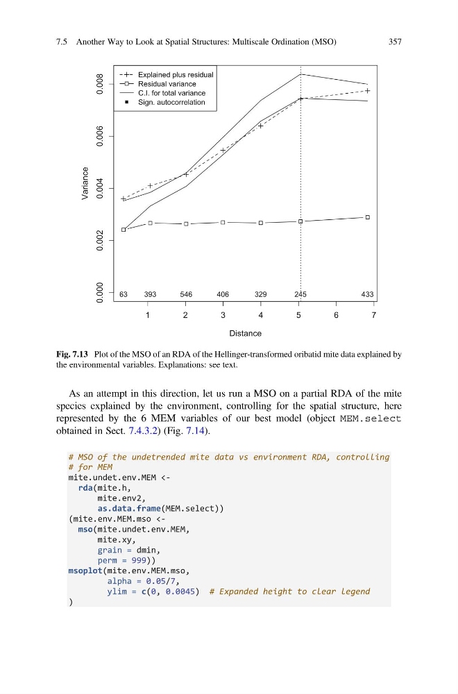
Fig. 7.13 Plot of the MSO of an RDA of the Hellinger-transformed oribatid mite data explained by
the environmental variables. Explanations: see text.
7.5 Another Way to Look at Spatial Structures: Multiscale Ordination (MSO)
357
species explained by the environment, controlling for the spatial structure, here
represented by the 6 MEM variables of our best model (object MEM.select
obtained in Sect. 7.4.3.2) (Fig. 7.14).
# MSO of the undetrended mite data vs environment RDA, controlling
# for MEM
mite.undet.env.MEM
as.data.frame(MEM.select))
(mite.env.MEM.mso
grain = dmin,
perm = 999))
msoplot(mite.env.MEM.mso,
alpha = 0.05/7,
ylim = c(0, 0.0045) # Expanded height to clear legend
)
1
2
3
4
5
6
7
0.000
0.002
0.004
0.006
0.008
Distance
Variance
Explained plus residual
Residual variance
C.I. for total variance
Sign. autocorrelation
63
393
546
406
329
433
245
Fig. 7.13 Plot of the MSO of an RDA of the Hellinger-transformed oribatid mite data explained by
the environmental variables. Explanations: see text.
7.5 Another Way to Look at Spatial Structures: Multiscale Ordination (MSO)
357