

from this threshold up to 4.0 m (i.e., approximately 4 times the threshold, used in the
dbMEM analysis).
# Construction of 10 neighbourhood matrices (class nb)
# Vector of 10 threshold distances
(thresh10 <- seq(give.thresh(dist(mite.xy)), 4, le = 10))
# Create 10 neighbourhood matrices.
# Each matrix contains all connexions with lengths smaller or equal
# to the threshold value
list10nb
x = as.matrix(mite.xy),
d1 = 0)
# Display an excerpt of the first neighbourhood matrix
print(
listw2mat(nb2listw(list10nb[[1]], style = "B"))[1:10, 1:10],
digits = 1
)
# Now we can apply the function test.W() to the 10 neighbourhood
# matrices. There are no weights on the links.
mite.thresh.res
Y = mite.h.det,
MEM.autocor = "positive")
)
# Lowest AICc, best model, threshold distance of best model
mite.thresh.minAIC
# Smallest AICc (best model among the 10)
min(mite.thresh.minAIC)
# Number of the model among the 10
which.min(mite.thresh.minAIC)
# Truncation threshold (distance)
thresh10[which.min(mite.thresh.minAIC)]
Hint dnearneigh() requires 2 geographic dimensions. Add a constant column (e.g.
a column of 1) if you only have 1 dimension, e.g. a transect or a time series.
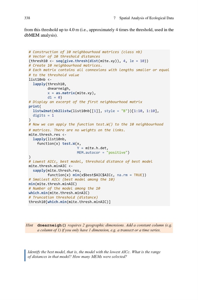
Identify the best model, that is, the model with the lowest AICc. What is the range
of distances in that model? How many MEMs were selected?
338
7 Spatial Analysis of Ecological Data
dbMEM analysis).
# Construction of 10 neighbourhood matrices (class nb)
# Vector of 10 threshold distances
(thresh10 <- seq(give.thresh(dist(mite.xy)), 4, le = 10))
# Create 10 neighbourhood matrices.
# Each matrix contains all connexions with lengths smaller or equal
# to the threshold value
list10nb
x = as.matrix(mite.xy),
d1 = 0)
# Display an excerpt of the first neighbourhood matrix
print(
listw2mat(nb2listw(list10nb[[1]], style = "B"))[1:10, 1:10],
digits = 1
)
# Now we can apply the function test.W() to the 10 neighbourhood
# matrices. There are no weights on the links.
mite.thresh.res
Y = mite.h.det,
MEM.autocor = "positive")
)
# Lowest AICc, best model, threshold distance of best model
mite.thresh.minAIC
# Smallest AICc (best model among the 10)
min(mite.thresh.minAIC)
# Number of the model among the 10
which.min(mite.thresh.minAIC)
# Truncation threshold (distance)
thresh10[which.min(mite.thresh.minAIC)]
Hint dnearneigh() requires 2 geographic dimensions. Add a constant column (e.g.
a column of 1) if you only have 1 dimension, e.g. a transect or a time series.
Identify the best model, that is, the model with the lowest AICc. What is the range
of distances in that model? How many MEMs were selected?
338
7 Spatial Analysis of Ecological Data