

The screen output says that the best model has an AICc value of -95.32 and is
based on 4 MEM variables.
# Unadjusted R^2 of best model
(R2.delW
RsquareAdj(
R2.delW,
n = nrow(mite.h.det),
m = which.min(mite.del.f2$best$AIC$AICc)
)
Third class of MEM model: connectivity matrix based on distances.
# 3a. Connectivity matrix based on a distance (radius around
#
points)
# Assessment of the relevant distances based on a multivariate
# variogram of the detrended mite data, with 20 distance classes.
(mite.vario <- variogmultiv(mite.h.det, mite.xy, nclass = 20))
plot(
mite.vario$d,
mite.vario$var,
ty = 'b',
pch = 20,
xlab = "Distance",
ylab = "C(distance)"
)
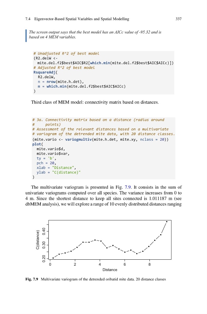
The multivariate variogram is presented in Fig. 7.9. It consists in the sum of
univariate variograms computed over all species. The variance increases from 0 to
4 m. Since the shortest distance to keep all sites connected is 1.011187 m (see
dbMEM analysis), we will explore a range of 10 evenly distributed distances ranging
0
2
4
6
8
0.20
0.30
0.40
Distance
C(distance)
Fig. 7.9 Multivariate variogram of the detrended oribatid mite data. 20 distance classes
7.4 Eigenvector-Based Spatial Variables and Spatial Modelling
337
based on 4 MEM variables.
# Unadjusted R^2 of best model
(R2.delW
RsquareAdj(
R2.delW,
n = nrow(mite.h.det),
m = which.min(mite.del.f2$best$AIC$AICc)
)
Third class of MEM model: connectivity matrix based on distances.
# 3a. Connectivity matrix based on a distance (radius around
#
points)
# Assessment of the relevant distances based on a multivariate
# variogram of the detrended mite data, with 20 distance classes.
(mite.vario <- variogmultiv(mite.h.det, mite.xy, nclass = 20))
plot(
mite.vario$d,
mite.vario$var,
ty = 'b',
pch = 20,
xlab = "Distance",
ylab = "C(distance)"
)
The multivariate variogram is presented in Fig. 7.9. It consists in the sum of
univariate variograms computed over all species. The variance increases from 0 to
4 m. Since the shortest distance to keep all sites connected is 1.011187 m (see
dbMEM analysis), we will explore a range of 10 evenly distributed distances ranging
0
2
4
6
8
0.20
0.30
0.40
Distance
C(distance)
Fig. 7.9 Multivariate variogram of the detrended oribatid mite data. 20 distance classes
7.4 Eigenvector-Based Spatial Variables and Spatial Modelling
337