

# Scalogram of the variance explained by all dbMEM eigenfunctions,
# computed with our homemade function scalog()
scalog(mite.dbmem.rda)
• Run forward selection and define submodels corresponding to groups of more or
less consecutive dbMEM variables retained by the procedure. This approach is
more conservative than the tests of significance in the scalogram because selection of explanatory variables stops when the adjusted R
2 of the global model is
reached..
• Draw maps of the significant dbMEM variables (Fig. 7.7) and group them
visually according to the scales of the patterns they represent:
# Maps of the 8 significant dbMEM variables with the homemade
# function sr.value()
par(mfrow = c(2, 4))
for(i in 1 : ncol(dbmem.red))
{
sr.value(mite.xy,
dbmem.red[ ,i],
sub = paste("dbMEM", dbmem.sign[i]),
csub = 2)
}
5
1 0
1 5
2 0
0.01 0.02 0.03 0.04
0.05 0.06
Scalogram
Eigenfunction number
R
2
p <= 0.001
p <= 0.01
p <= 0.05
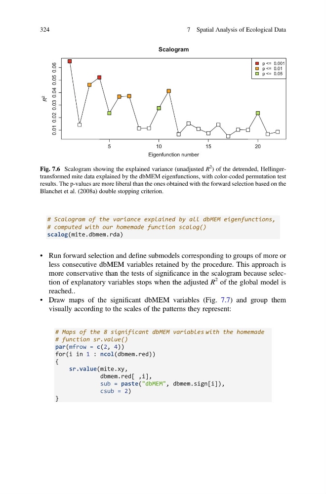
Fig. 7.6 Scalogram showing the explained variance (unadjusted R
2
) of the detrended, Hellingertransformed mite data explained by the dbMEM eigenfunctions, with color-coded permutation test
results. The p-values are more liberal than the ones obtained with the forward selection based on the
Blanchet et al. (2008a) double stopping criterion.
324
7 Spatial Analysis of Ecological Data
# computed with our homemade function scalog()
scalog(mite.dbmem.rda)
• Run forward selection and define submodels corresponding to groups of more or
less consecutive dbMEM variables retained by the procedure. This approach is
more conservative than the tests of significance in the scalogram because selection of explanatory variables stops when the adjusted R
2 of the global model is
reached..
• Draw maps of the significant dbMEM variables (Fig. 7.7) and group them
visually according to the scales of the patterns they represent:
# Maps of the 8 significant dbMEM variables with the homemade
# function sr.value()
par(mfrow = c(2, 4))
for(i in 1 : ncol(dbmem.red))
{
sr.value(mite.xy,
dbmem.red[ ,i],
sub = paste("dbMEM", dbmem.sign[i]),
csub = 2)
}
5
1 0
1 5
2 0
0.01 0.02 0.03 0.04
0.05 0.06
Scalogram
Eigenfunction number
R
2
p <= 0.001
p <= 0.01
p <= 0.05
Fig. 7.6 Scalogram showing the explained variance (unadjusted R
2
) of the detrended, Hellingertransformed mite data explained by the dbMEM eigenfunctions, with color-coded permutation test
results. The p-values are more liberal than the ones obtained with the forward selection based on the
Blanchet et al. (2008a) double stopping criterion.
324
7 Spatial Analysis of Ecological Data