

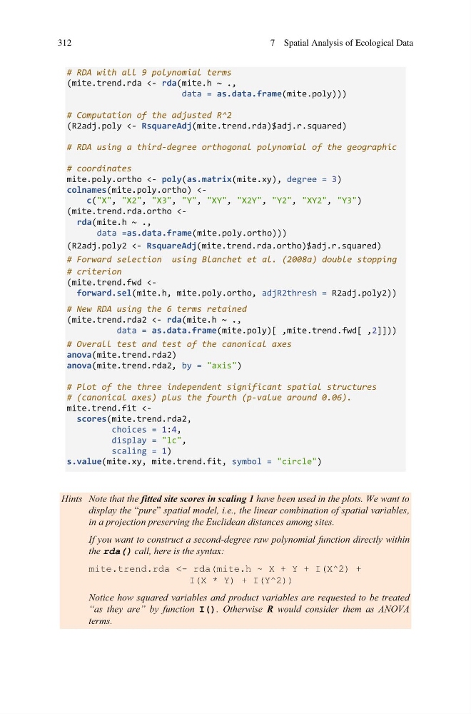
# RDA with all 9 polynomial terms
(mite.trend.rda <- rda(mite.h ~ .,
data = as.data.frame(mite.poly)))
# Computation of the adjusted R^2
(R2adj.poly <- RsquareAdj(mite.trend.rda)$adj.r.squared)
# RDA using a third-degree orthogonal polynomial of the geographic
# coordinates
mite.poly.ortho <- poly(as.matrix(mite.xy), degree = 3)
colnames(mite.poly.ortho)
(R2adj.poly2 <- RsquareAdj(mite.trend.rda.ortho)$adj.r.squared)
# Forward selection using Blanchet et al. (2008a) double stopping
# criterion
(mite.trend.fwd
# New RDA using the 6 terms retained
(mite.trend.rda2 <- rda(mite.h ~ .,
data = as.data.frame(mite.poly)[ ,mite.trend.fwd[ ,2]]))
# Overall test and test of the canonical axes
anova(mite.trend.rda2)
anova(mite.trend.rda2, by = "axis")
# Plot of the three independent significant spatial structures
# (canonical axes) plus the fourth (p-value around 0.06).
mite.trend.fit
display = "lc",
scaling = 1)
s.value(mite.xy, mite.trend.fit, symbol = "circle")
Hints Note that the fitted site scores in scaling 1 have been used in the plots. We want to
display the “pure” spatial model, i.e., the linear combination of spatial variables,
in a projection preserving the Euclidean distances among sites.
If you want to construct a second-degree raw polynomial function directly within
the rda() call, here is the syntax:
mite.trend.rda <- rda(mite.h ~ X + Y + I(X^2) +
I(X * Y) + I(Y^2))
Notice how squared variables and product variables are requested to be treated
“as they are” by function I(). Otherwise R would consider them as ANOVA
terms.
312
7 Spatial Analysis of Ecological Data
(mite.trend.rda <- rda(mite.h ~ .,
data = as.data.frame(mite.poly)))
# Computation of the adjusted R^2
(R2adj.poly <- RsquareAdj(mite.trend.rda)$adj.r.squared)
# RDA using a third-degree orthogonal polynomial of the geographic
# coordinates
mite.poly.ortho <- poly(as.matrix(mite.xy), degree = 3)
colnames(mite.poly.ortho)
(R2adj.poly2 <- RsquareAdj(mite.trend.rda.ortho)$adj.r.squared)
# Forward selection using Blanchet et al. (2008a) double stopping
# criterion
(mite.trend.fwd
(mite.trend.rda2 <- rda(mite.h ~ .,
data = as.data.frame(mite.poly)[ ,mite.trend.fwd[ ,2]]))
# Overall test and test of the canonical axes
anova(mite.trend.rda2)
anova(mite.trend.rda2, by = "axis")
# Plot of the three independent significant spatial structures
# (canonical axes) plus the fourth (p-value around 0.06).
mite.trend.fit
display = "lc",
scaling = 1)
s.value(mite.xy, mite.trend.fit, symbol = "circle")
Hints Note that the fitted site scores in scaling 1 have been used in the plots. We want to
display the “pure” spatial model, i.e., the linear combination of spatial variables,
in a projection preserving the Euclidean distances among sites.
If you want to construct a second-degree raw polynomial function directly within
the rda() call, here is the syntax:
mite.trend.rda <- rda(mite.h ~ X + Y + I(X^2) +
I(X * Y) + I(Y^2))
Notice how squared variables and product variables are requested to be treated
“as they are” by function I(). Otherwise R would consider them as ANOVA
terms.
312
7 Spatial Analysis of Ecological Data