Note that the points do not form a connected graph at this radius. Following that, the
function sp.correlogram() will find successive lag orders of contiguous neighbours and compute Moran’s I for each of these lag orders. A lag order is the number of
links, or steps in the linkage graph, between two points. It can be construed as a
generalized form of distance between points. For instance, if sites A and C are
connected through site B, two links (A-B and B-C) are needed to connect A and C,
which are then are connected at lag order 2.
Note: Cartesian coordinates can be obtained from latitude-longitude (sometimes
abbreviated to Lat/Lon or LatLon) data using the function geoXY() of the
package SoDA.
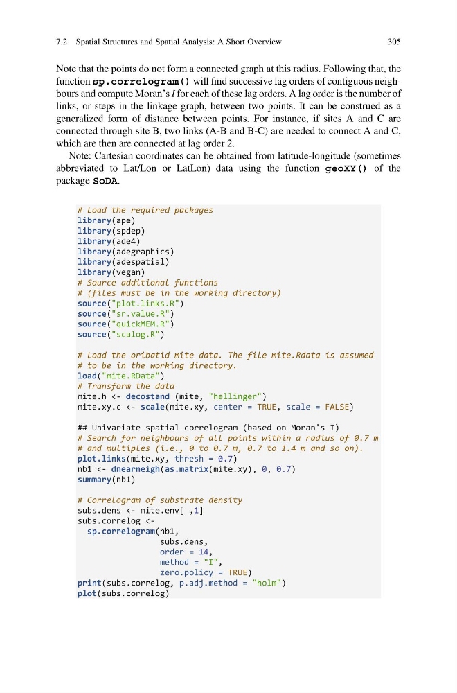
# Load the required packages
library(ape)
library(spdep)
library(ade4)
library(adegraphics)
library(adespatial)
library(vegan)
# Source additional functions
# (files must be in the working directory)
source("plot.links.R")
source("sr.value.R")
source("quickMEM.R")
source("scalog.R")
# Load the oribatid mite data. The file mite.Rdata is assumed
# to be in the working directory.
load("mite.RData")
# Transform the data
mite.h <- decostand (mite, "hellinger")
mite.xy.c <- scale(mite.xy, center = TRUE, scale = FALSE)
## Univariate spatial correlogram (based on Moran's I)
# Search for neighbours of all points within a radius of 0.7 m
# and multiples (i.e., 0 to 0.7 m, 0.7 to 1.4 m and so on).
plot.links(mite.xy, thresh = 0.7)
nb1 <- dnearneigh(as.matrix(mite.xy), 0, 0.7)
summary(nb1)
# Correlogram of substrate density
subs.dens <- mite.env[ ,1]
subs.correlog subs.dens,
order = 14,
method = "I",
zero.policy = TRUE)
print(subs.correlog, p.adj.method = "holm")
plot(subs.correlog)
7.2 Spatial Structures and Spatial Analysis: A Short Overview
305