

7.2.2 Induced Spatial Dependence and Spatial
Autocorrelation
An important distinction must be made here. As we wrote above, a spatial structure
in a response matrix Y can result from two main origins: either from the forcing of
external (environmental) factors that are themselves spatially structured, or as the
result of processes internal to the community itself. In the first case one speaks of
induced spatial dependence, in the second case of spatial autocorrelation.
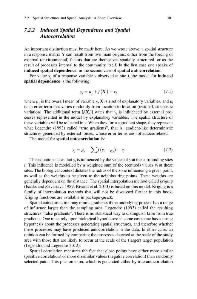
For value y j of a response variable y observed at site j, the model for induced
spatial dependence is the following:
y j ¼ μ y þ f X j
À Á þ ε j
ð7:1Þ
where μ y is the overall mean of variable y, X is a set of explanatory variables, and ε j
is an error term that varies randomly from location to location (residual, stochastic
variation). The additional term [f(X i )] states that y j is influenced by external processes represented in the model by explanatory variables. The spatial structure of
these variables will be reflected in y. When they form a gradient shape, they represent
what Legendre (1993) called “true gradients”, that is, gradient-like deterministic
structures generated by external forces, whose error terms are not autocorrelated.
The model for spatial autocorrelation is:
y j ¼ μ y þ
X
f y i À μ y
À
Á þ ε j
ð7:2Þ
This equation states that y j is influenced by the values of y at the surrounding sites
i. This influence is modelled by a weighted sum of the (centred) values y i at these
sites. The biological context dictates the radius of the zone influencing a given point,
as well as the weights to be given to the neighbouring points. These weights are
generally dependent on the distance. The spatial interpolation method called kriging
(Isaaks and Srivastava 1989; Bivand et al. 2013) is based on this model. Kriging is a
family of interpolation methods that will not be discussed further in this book.
Kriging functions are available in package geoR.
Spatial autocorrelation may mimic gradients if the underlying process has a range
of influence larger than the sampling area. Legendre (1993) called the resulting
structures “false gradients”. There is no statistical way to distinguish false from true
gradients. One must rely upon biological hypotheses: in some cases one has a strong
hypothesis about the processes generating spatial structures, and therefore whether
these processes may have produced autocorrelation in the data. In other cases an
opinion can be formed by comparing the processes detected at the scale of the study
area with those that are likely to occur at the scale of the (larger) target population
(Legendre and Legendre 2012).
Spatial correlation measures the fact that close points have either more similar
(positive correlation) or more dissimilar values (negative correlation) than randomly
selected pairs. This phenomenon, which is generated either by true autocorrelation
7.2 Spatial Structures and Spatial Analysis: A Short Overview
301
Autocorrelation
An important distinction must be made here. As we wrote above, a spatial structure
in a response matrix Y can result from two main origins: either from the forcing of
external (environmental) factors that are themselves spatially structured, or as the
result of processes internal to the community itself. In the first case one speaks of
induced spatial dependence, in the second case of spatial autocorrelation.
For value y j of a response variable y observed at site j, the model for induced
spatial dependence is the following:
y j ¼ μ y þ f X j
À Á þ ε j
ð7:1Þ
where μ y is the overall mean of variable y, X is a set of explanatory variables, and ε j
is an error term that varies randomly from location to location (residual, stochastic
variation). The additional term [f(X i )] states that y j is influenced by external processes represented in the model by explanatory variables. The spatial structure of
these variables will be reflected in y. When they form a gradient shape, they represent
what Legendre (1993) called “true gradients”, that is, gradient-like deterministic
structures generated by external forces, whose error terms are not autocorrelated.
The model for spatial autocorrelation is:
y j ¼ μ y þ
X
f y i À μ y
À
Á þ ε j
ð7:2Þ
This equation states that y j is influenced by the values of y at the surrounding sites
i. This influence is modelled by a weighted sum of the (centred) values y i at these
sites. The biological context dictates the radius of the zone influencing a given point,
as well as the weights to be given to the neighbouring points. These weights are
generally dependent on the distance. The spatial interpolation method called kriging
(Isaaks and Srivastava 1989; Bivand et al. 2013) is based on this model. Kriging is a
family of interpolation methods that will not be discussed further in this book.
Kriging functions are available in package geoR.
Spatial autocorrelation may mimic gradients if the underlying process has a range
of influence larger than the sampling area. Legendre (1993) called the resulting
structures “false gradients”. There is no statistical way to distinguish false from true
gradients. One must rely upon biological hypotheses: in some cases one has a strong
hypothesis about the processes generating spatial structures, and therefore whether
these processes may have produced autocorrelation in the data. In other cases an
opinion can be formed by comparing the processes detected at the scale of the study
area with those that are likely to occur at the scale of the (larger) target population
(Legendre and Legendre 2012).
Spatial correlation measures the fact that close points have either more similar
(positive correlation) or more dissimilar values (negative correlation) than randomly
selected pairs. This phenomenon, which is generated either by true autocorrelation
7.2 Spatial Structures and Spatial Analysis: A Short Overview
301