

The posterior probabilities of the new objects (rows) to belong to groups 1–4
(columns) are given by element “$posterior” of the prediction result. Here the
result is:
$posterior
1
2
3
4
1 0.1118150083 0.8879697 0.0002152868 2.067257e-09
2 0.0009074883 0.1115628 0.8875164034 1.328932e-05
The first object (row 1) has the highest probability (0.88) to belong to group
2, and the second object to group 3. Now you could examine the profiles of the fish
species of groups 2 and 3. What you have actually done is to forecast that a site with
the environmental values written in data frame newo should contain this type of fish
community.
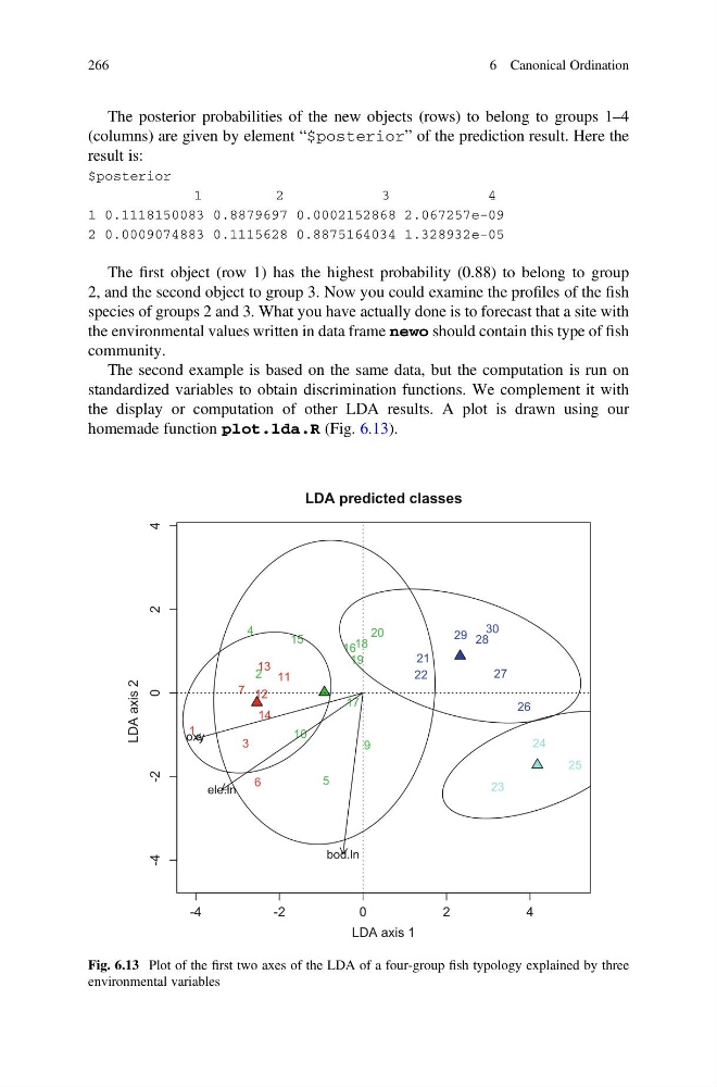
The second example is based on the same data, but the computation is run on
standardized variables to obtain discrimination functions. We complement it with
the display or computation of other LDA results. A plot is drawn using our
homemade function plot.lda.R (Fig. 6.13).
-4
-2
0
2
4
-4
-2
0
2
4
LDA predicted classes
LDA axis 1
LDA axis 2
1
2
3
4
5
6
7
9
10
11
12
13
14
15
16
17
18
19
20
21
22
23
24
25
26
27
28
29
30
ele.ln
oxy
bod.ln
Fig. 6.13 Plot of the first two axes of the LDA of a four-group fish typology explained by three
environmental variables
266
6 Canonical Ordination
(columns) are given by element “$posterior” of the prediction result. Here the
result is:
$posterior
1
2
3
4
1 0.1118150083 0.8879697 0.0002152868 2.067257e-09
2 0.0009074883 0.1115628 0.8875164034 1.328932e-05
The first object (row 1) has the highest probability (0.88) to belong to group
2, and the second object to group 3. Now you could examine the profiles of the fish
species of groups 2 and 3. What you have actually done is to forecast that a site with
the environmental values written in data frame newo should contain this type of fish
community.
The second example is based on the same data, but the computation is run on
standardized variables to obtain discrimination functions. We complement it with
the display or computation of other LDA results. A plot is drawn using our
homemade function plot.lda.R (Fig. 6.13).
-4
-2
0
2
4
-4
-2
0
2
4
LDA predicted classes
LDA axis 1
LDA axis 2
1
2
3
4
5
6
7
9
10
11
12
13
14
15
16
17
18
19
20
21
22
23
24
25
26
27
28
29
30
ele.ln
oxy
bod.ln
Fig. 6.13 Plot of the first two axes of the LDA of a four-group fish typology explained by three
environmental variables
266
6 Canonical Ordination