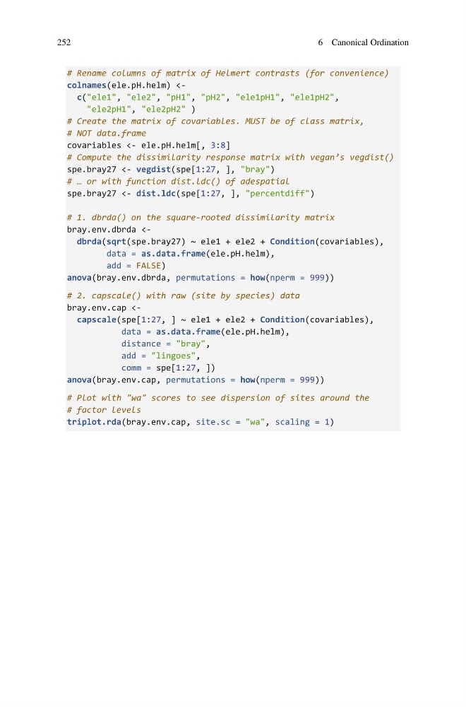
# Rename columns of matrix of Helmert contrasts (for convenience)
colnames(ele.pH.helm) "ele2pH1", "ele2pH2" )
# Create the matrix of covariables. MUST be of class matrix,
# NOT data.frame
covariables <- ele.pH.helm[, 3:8]
# Compute the dissimilarity response matrix with vegan’s vegdist()
spe.bray27 <- vegdist(spe[1:27, ], "bray")
# … or with function dist.ldc() of adespatial
spe.bray27 <- dist.ldc(spe[1:27, ], "percentdiff")
# 1. dbrda() on the square-rooted dissimilarity matrix
bray.env.dbrda data = as.data.frame(ele.pH.helm),
add = FALSE)
anova(bray.env.dbrda, permutations = how(nperm = 999))
# 2. capscale() with raw (site by species) data
bray.env.cap data = as.data.frame(ele.pH.helm),
distance = "bray",
add = "lingoes",
comm = spe[1:27, ])
anova(bray.env.cap, permutations = how(nperm = 999))
# Plot with "wa" scores to see dispersion of sites around the
# factor levels
triplot.rda(bray.env.cap, site.sc = "wa", scaling = 1)
252
6 Canonical Ordination