

test is to generate a reference distribution of the chosen statistic under the null
hypothesis H 0 by randomly permuting appropriate elements of the data a large
number of times and recomputing the statistic each time. Then one compares the
true value of the statistic to this reference distribution. The p-value is computed as
the proportion of the permuted values equal to or larger than the true (unpermuted)
value of the statistic for a one-tailed test in the upper tail, like the F-test used in RDA.
The true value is included in this count. The null hypothesis is rejected if this p-value
is equal to or smaller than the predefined significance level α.
Three elements are critical in the construction of a permutation test: (1) the choice
of the permutable units, (2) the choice of the statistic, and (3) the permutation
scheme.
The permutable units are often the response data (random permutation of the
rows of the Y data matrix), but sometimes other permutable units must be defined. In
partial canonical analysis (Sect. 6.3.2.5), for example, it is the residuals of some
regression model that are permuted. See Legendre and Legendre (2012, pp. 651 et
sq. and especially Table 11.6 p. 653). In the simple case presented here, the null
hypothesis H 0 states (loosely) that no (linear) relationship exists between the
response data Y and the explanatory variables X. In terms of permutation tests,
this means that the sites in matrix Y can be permuted randomly to produce realizations of this H 0 , thereby destroying the possible relationship between a given fish
assemblage and the ecological condition of its site. A permutation test repeats the
calculation with permuted datas 100, 1000 or 10,000 times (including the true,
unpermuted value) to produce a large sample of test statistics to which the true
value is compared.
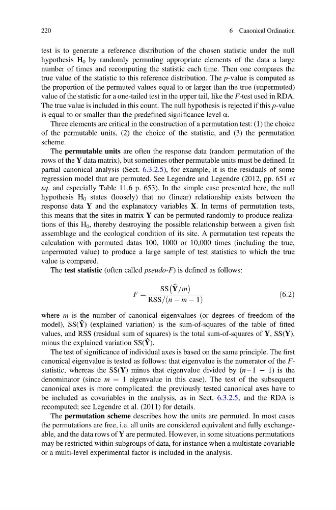
The test statistic (often called pseudo-F) is defined as follows:
F ¼
SS
À b
Y=m
Á
RSS= n À m À 1
ð
Þ
ð6:2Þ
where m is the number of canonical eigenvalues (or degrees of freedom of the
model), SS(Ŷ) (explained variation) is the sum-of-squares of the table of fitted
values, and RSS (residual sum of squares) is the total sum-of-squares of Y, SS(Y),
minus the explained variation SS(Ŷ).
The test of significance of individual axes is based on the same principle. The first
canonical eigenvalue is tested as follows: that eigenvalue is the numerator of the Fstatistic, whereas the SS(Y) minus that eigenvalue divided by (n – 1 À 1) is the
denominator (since m ¼ 1 eigenvalue in this case). The test of the subsequent
canonical axes is more complicated: the previously tested canonical axes have to
be included as covariables in the analysis, as in Sect. 6.3.2.5, and the RDA is
recomputed; see Legendre et al. (2011) for details.
The permutation scheme describes how the units are permuted. In most cases
the permutations are free, i.e. all units are considered equivalent and fully exchangeable, and the data rows of Y are permuted. However, in some situations permutations
may be restricted within subgroups of data, for instance when a multistate covariable
or a multi-level experimental factor is included in the analysis.
220
6 Canonical Ordination
hypothesis H 0 by randomly permuting appropriate elements of the data a large
number of times and recomputing the statistic each time. Then one compares the
true value of the statistic to this reference distribution. The p-value is computed as
the proportion of the permuted values equal to or larger than the true (unpermuted)
value of the statistic for a one-tailed test in the upper tail, like the F-test used in RDA.
The true value is included in this count. The null hypothesis is rejected if this p-value
is equal to or smaller than the predefined significance level α.
Three elements are critical in the construction of a permutation test: (1) the choice
of the permutable units, (2) the choice of the statistic, and (3) the permutation
scheme.
The permutable units are often the response data (random permutation of the
rows of the Y data matrix), but sometimes other permutable units must be defined. In
partial canonical analysis (Sect. 6.3.2.5), for example, it is the residuals of some
regression model that are permuted. See Legendre and Legendre (2012, pp. 651 et
sq. and especially Table 11.6 p. 653). In the simple case presented here, the null
hypothesis H 0 states (loosely) that no (linear) relationship exists between the
response data Y and the explanatory variables X. In terms of permutation tests,
this means that the sites in matrix Y can be permuted randomly to produce realizations of this H 0 , thereby destroying the possible relationship between a given fish
assemblage and the ecological condition of its site. A permutation test repeats the
calculation with permuted datas 100, 1000 or 10,000 times (including the true,
unpermuted value) to produce a large sample of test statistics to which the true
value is compared.
The test statistic (often called pseudo-F) is defined as follows:
F ¼
SS
À b
Y=m
Á
RSS= n À m À 1
ð
Þ
ð6:2Þ
where m is the number of canonical eigenvalues (or degrees of freedom of the
model), SS(Ŷ) (explained variation) is the sum-of-squares of the table of fitted
values, and RSS (residual sum of squares) is the total sum-of-squares of Y, SS(Y),
minus the explained variation SS(Ŷ).
The test of significance of individual axes is based on the same principle. The first
canonical eigenvalue is tested as follows: that eigenvalue is the numerator of the Fstatistic, whereas the SS(Y) minus that eigenvalue divided by (n – 1 À 1) is the
denominator (since m ¼ 1 eigenvalue in this case). The test of the subsequent
canonical axes is more complicated: the previously tested canonical axes have to
be included as covariables in the analysis, as in Sect. 6.3.2.5, and the RDA is
recomputed; see Legendre et al. (2011) for details.
The permutation scheme describes how the units are permuted. In most cases
the permutations are free, i.e. all units are considered equivalent and fully exchangeable, and the data rows of Y are permuted. However, in some situations permutations
may be restricted within subgroups of data, for instance when a multistate covariable
or a multi-level experimental factor is included in the analysis.
220
6 Canonical Ordination