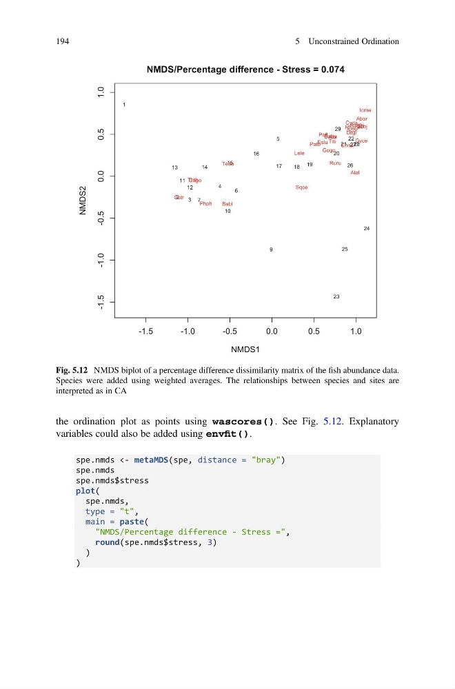
the ordination plot as points using wascores(). See Fig. 5.12. Explanatory
variables could also be added using envfit().
spe.nmds <- metaMDS(spe, distance = "bray")
spe.nmds
spe.nmds$stress
plot(
spe.nmds,
type = "t",
main = paste(
"NMDS/Percentage difference - Stress =",
round(spe.nmds$stress, 3)
)
)
-1.5
-1.0
-0.5
0.0
0.5
1.0
-1.5
-1.0
-0.5
0.0
0.5
1.0
NMDS/Percentage difference - Stress = 0.074
NMDS1
NMDS2
1
2
3
4
5
6
7
9
10
11
12
13
14
15
16
17
18 19
20
21
22
23
24
25
26
27 28
29
30
Cogo
Satr
Phph
Babl
Thth
Teso
Chna
Pato
Lele
Sqce
Baba Albi
Gogo
Eslu
Pefl
Rham
Legi Scer
Cyca
Titi
Abbr
Icme
Gyce
Ruru
Blbj
Alal
Anan
Fig. 5.12 NMDS biplot of a percentage difference dissimilarity matrix of the fish abundance data.
Species were added using weighted averages. The relationships between species and sites are
interpreted as in CA
194
5 Unconstrained Ordination