

As mentioned above, PCoA should actually be reserved to situations where no
Euclidean measure is available or selected. With Jaccard and Sørensen dissimilarity
matrices computed by ade4, for example, the ordination is fully Euclidean because
ade4 takes the square root of the dissimilarities. In other cases, however, such as
percentage difference dissimilarities computed with vegan (method¼"bray"),
the dissimilarity matrices may not be Euclidean (see Sect. 3.3). This results in PCoA
producing some negative eigenvalues. Lingoes and Cailliez corrections are available
in the function pcoa(). This function provides the eigenvalues along with a
broken stick comparison in its output. In the examples below, when a correction is
requested for, the second column contains the corrected eigenvalues. However, the
easiest way of obtaining a fully Euclidean ordination solution remains to take the
square root of the dissimilarities before computing PCoA.
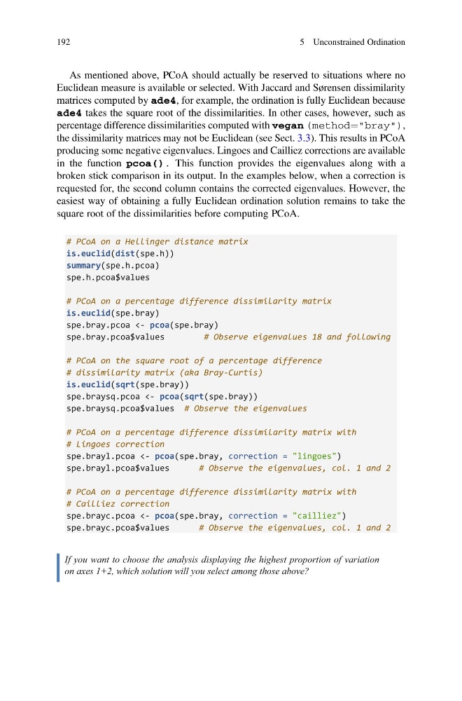
# PCoA on a percentage difference dissimilarity matrix
is.euclid(spe.bray)
spe.bray.pcoa <- pcoa(spe.bray)
spe.bray.pcoa$values
# Observe eigenvalues 18 and following
# PCoA on the square root of a percentage difference
# dissimilarity matrix (aka Bray-Curtis)
is.euclid(sqrt(spe.bray))
spe.braysq.pcoa <- pcoa(sqrt(spe.bray))
spe.braysq.pcoa$values # Observe the eigenvalues
# PCoA on a percentage difference dissimilarity matrix with
# Lingoes correction
spe.brayl.pcoa <- pcoa(spe.bray, correction = "lingoes")
spe.brayl.pcoa$values
# Observe the eigenvalues, col. 1 and 2
# PCoA on a percentage difference dissimilarity matrix with
# Cailliez correction
spe.brayc.pcoa <- pcoa(spe.bray, correction = "cailliez")
spe.brayc.pcoa$values
# Observe the eigenvalues, col. 1 and 2
# PCoA on a Hellinger distance matrix
is.euclid(dist(spe.h))
summary(spe.h.pcoa)
spe.h.pcoa$values
If you want to choose the analysis displaying the highest proportion of variation
on axes 1+2, which solution will you select among those above?
192
5 Unconstrained Ordination
Euclidean measure is available or selected. With Jaccard and Sørensen dissimilarity
matrices computed by ade4, for example, the ordination is fully Euclidean because
ade4 takes the square root of the dissimilarities. In other cases, however, such as
percentage difference dissimilarities computed with vegan (method¼"bray"),
the dissimilarity matrices may not be Euclidean (see Sect. 3.3). This results in PCoA
producing some negative eigenvalues. Lingoes and Cailliez corrections are available
in the function pcoa(). This function provides the eigenvalues along with a
broken stick comparison in its output. In the examples below, when a correction is
requested for, the second column contains the corrected eigenvalues. However, the
easiest way of obtaining a fully Euclidean ordination solution remains to take the
square root of the dissimilarities before computing PCoA.
# PCoA on a percentage difference dissimilarity matrix
is.euclid(spe.bray)
spe.bray.pcoa <- pcoa(spe.bray)
spe.bray.pcoa$values
# Observe eigenvalues 18 and following
# PCoA on the square root of a percentage difference
# dissimilarity matrix (aka Bray-Curtis)
is.euclid(sqrt(spe.bray))
spe.braysq.pcoa <- pcoa(sqrt(spe.bray))
spe.braysq.pcoa$values # Observe the eigenvalues
# PCoA on a percentage difference dissimilarity matrix with
# Lingoes correction
spe.brayl.pcoa <- pcoa(spe.bray, correction = "lingoes")
spe.brayl.pcoa$values
# Observe the eigenvalues, col. 1 and 2
# PCoA on a percentage difference dissimilarity matrix with
# Cailliez correction
spe.brayc.pcoa <- pcoa(spe.bray, correction = "cailliez")
spe.brayc.pcoa$values
# Observe the eigenvalues, col. 1 and 2
# PCoA on a Hellinger distance matrix
is.euclid(dist(spe.h))
summary(spe.h.pcoa)
spe.h.pcoa$values
If you want to choose the analysis displaying the highest proportion of variation
on axes 1+2, which solution will you select among those above?
192
5 Unconstrained Ordination