

shares the “Barepeat” modality and the pair 21 + 26 shares the “Sphagn4”
modality. These two modalities have only two occurrences in the data set. These
results show that MCA shares with CA the property of emphasizing rare events,
which may be useful to identify rare characteristics or otherwise special features in a
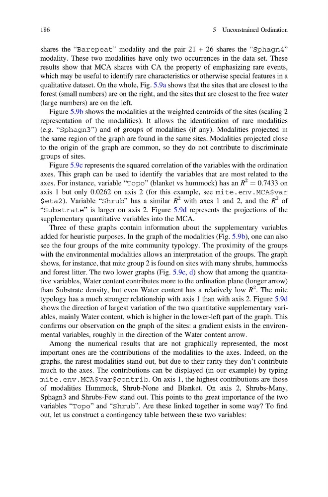
qualitative dataset. On the whole, Fig. 5.9a shows that the sites that are closest to the
forest (small numbers) are on the right, and the sites that are closest to the free water
(large numbers) are on the left.
Figure 5.9b shows the modalities at the weighted centroids of the sites (scaling 2
representation of the modalities). It allows the identification of rare modalities
(e.g. “Sphagn3”) and of groups of modalities (if any). Modalities projected in
the same region of the graph are found in the same sites. Modalities projected close
to the origin of the graph are common, so they do not contribute to discriminate
groups of sites.
Figure 5.9c represents the squared correlation of the variables with the ordination
axes. This graph can be used to identify the variables that are most related to the
axes. For instance, variable “Topo” (blanket vs hummock) has an R
2
¼ 0.7433 on
axis 1 but only 0.0262 on axis 2 (for this example, see mite.env.MCA$var
$eta2). Variable “Shrub” has a similar R
2 with axes 1 and 2, and the R
2 of
“Substrate” is larger on axis 2. Figure 5.9d represents the projections of the
supplementary quantitative variables into the MCA.
Three of these graphs contain information about the supplementary variables
added for heuristic purposes. In the graph of the modalities (Fig. 5.9b), one can also
see the four groups of the mite community typology. The proximity of the groups
with the environmental modalities allows an interpretation of the groups. The graph
shows, for instance, that mite group 2 is found on sites with many shrubs, hummocks
and forest litter. The two lower graphs (Fig. 5.9c, d) show that among the quantitative variables, Water content contributes more to the ordination plane (longer arrow)
than Substrate density, but even Water content has a relatively low R
2 . The mite
typology has a much stronger relationship with axis 1 than with axis 2. Figure 5.9d
shows the direction of largest variation of the two quantitative supplementary variables, mainly Water content, which is higher in the lower-left part of the graph. This
confirms our observation on the graph of the sites: a gradient exists in the environmental variables, roughly in the direction of the Water content arrow.
Among the numerical results that are not graphically represented, the most
important ones are the contributions of the modalities to the axes. Indeed, on the
graphs, the rarest modalities stand out, but due to their rarity they don’t contribute
much to the axes. The contributions can be displayed (in our example) by typing
mite.env.MCA$var$contrib. On axis 1, the highest contributions are those
of modalities Hummock, Shrub-None and Blanket. On axis 2, Shrubs-Many,
Sphagn3 and Shrubs-Few stand out. This points to the great importance of the two
variables “Topo” and “Shrub”. Are these linked together in some way? To find
out, let us construct a contingency table between these two variables:
186
5 Unconstrained Ordination
modality. These two modalities have only two occurrences in the data set. These
results show that MCA shares with CA the property of emphasizing rare events,
which may be useful to identify rare characteristics or otherwise special features in a
qualitative dataset. On the whole, Fig. 5.9a shows that the sites that are closest to the
forest (small numbers) are on the right, and the sites that are closest to the free water
(large numbers) are on the left.
Figure 5.9b shows the modalities at the weighted centroids of the sites (scaling 2
representation of the modalities). It allows the identification of rare modalities
(e.g. “Sphagn3”) and of groups of modalities (if any). Modalities projected in
the same region of the graph are found in the same sites. Modalities projected close
to the origin of the graph are common, so they do not contribute to discriminate
groups of sites.
Figure 5.9c represents the squared correlation of the variables with the ordination
axes. This graph can be used to identify the variables that are most related to the
axes. For instance, variable “Topo” (blanket vs hummock) has an R
2
¼ 0.7433 on
axis 1 but only 0.0262 on axis 2 (for this example, see mite.env.MCA$var
$eta2). Variable “Shrub” has a similar R
2 with axes 1 and 2, and the R
2 of
“Substrate” is larger on axis 2. Figure 5.9d represents the projections of the
supplementary quantitative variables into the MCA.
Three of these graphs contain information about the supplementary variables
added for heuristic purposes. In the graph of the modalities (Fig. 5.9b), one can also
see the four groups of the mite community typology. The proximity of the groups
with the environmental modalities allows an interpretation of the groups. The graph
shows, for instance, that mite group 2 is found on sites with many shrubs, hummocks
and forest litter. The two lower graphs (Fig. 5.9c, d) show that among the quantitative variables, Water content contributes more to the ordination plane (longer arrow)
than Substrate density, but even Water content has a relatively low R
2 . The mite
typology has a much stronger relationship with axis 1 than with axis 2. Figure 5.9d
shows the direction of largest variation of the two quantitative supplementary variables, mainly Water content, which is higher in the lower-left part of the graph. This
confirms our observation on the graph of the sites: a gradient exists in the environmental variables, roughly in the direction of the Water content arrow.
Among the numerical results that are not graphically represented, the most
important ones are the contributions of the modalities to the axes. Indeed, on the
graphs, the rarest modalities stand out, but due to their rarity they don’t contribute
much to the axes. The contributions can be displayed (in our example) by typing
mite.env.MCA$var$contrib. On axis 1, the highest contributions are those
of modalities Hummock, Shrub-None and Blanket. On axis 2, Shrubs-Many,
Sphagn3 and Shrubs-Few stand out. This points to the great importance of the two
variables “Topo” and “Shrub”. Are these linked together in some way? To find
out, let us construct a contingency table between these two variables:
186
5 Unconstrained Ordination