

(GAM). For this example, let us retain variables discharge (dis) and ammonium
(amm), since both are important and are not overly correlated, as seen in Fig. 5.2. The
resulting object will be used as in Sect. 5.3.3.2, but then we will add the fitted
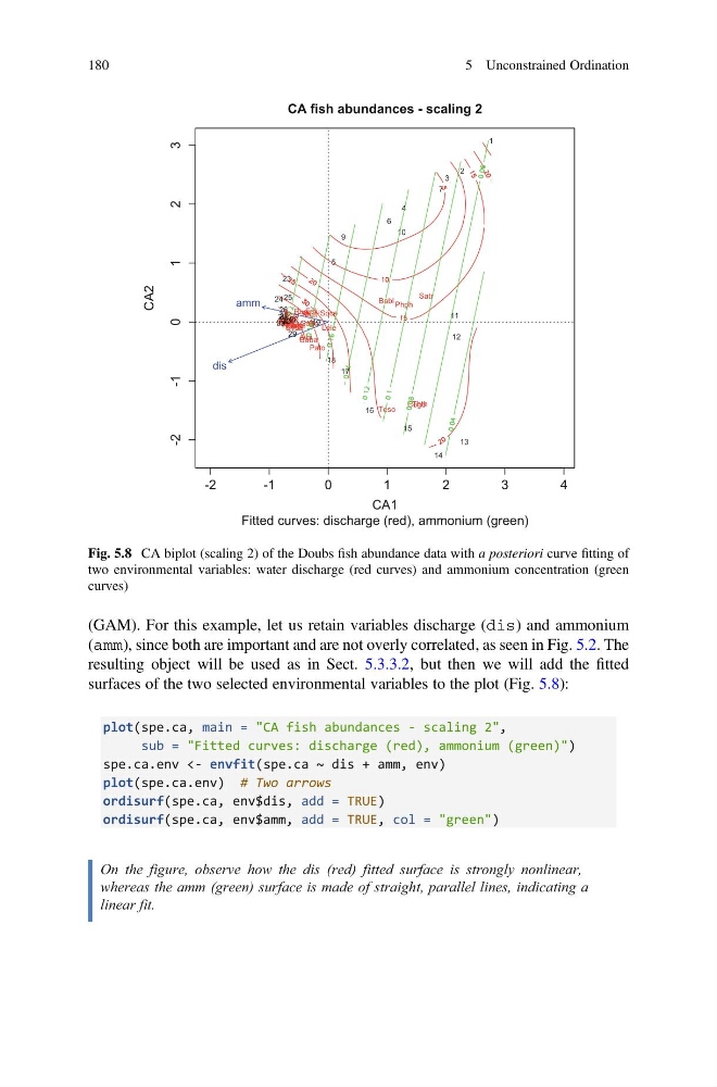
surfaces of the two selected environmental variables to the plot (Fig. 5.8):
plot(spe.ca, main = "CA fish abundances - scaling 2",
sub = "Fitted curves: discharge (red), ammonium (green)")
spe.ca.env <- envfit(spe.ca ~ dis + amm, env)
plot(spe.ca.env) # Two arrows
ordisurf(spe.ca, env$dis, add = TRUE)
ordisurf(spe.ca, env$amm, add = TRUE, col = "green")
On the figure, observe how the dis (red) fitted surface is strongly nonlinear,
whereas the amm (green) surface is made of straight, parallel lines, indicating a
linear fit.
-2
-1
0
1
2
3
4
-2
-1
0
1
2
3
CA fish abundances - scaling 2
CA1
Fitted curves: discharge (red), ammonium (green)
CA2
Cogo
Satr
Phph
Babl
Thth
Teso
Chna
Pato
Lele
Sqce
Baba
Albi
Gogo
Eslu
Pefl
Rham Legi
Scer
Cyca
Titi
Abbr
Icme Gyce
Ruru
Blbj Alal
Anan
1
2
3
4
5
6
7
9
10
11
12
13
14
15
16
17
18
19
20
21
22
23
24 25
26
27
28
29
30
dis
amm
Fig. 5.8 CA biplot (scaling 2) of the Doubs fish abundance data with a posteriori curve fitting of
two environmental variables: water discharge (red curves) and ammonium concentration (green
curves)
180
5 Unconstrained Ordination
(amm), since both are important and are not overly correlated, as seen in Fig. 5.2. The
resulting object will be used as in Sect. 5.3.3.2, but then we will add the fitted
surfaces of the two selected environmental variables to the plot (Fig. 5.8):
plot(spe.ca, main = "CA fish abundances - scaling 2",
sub = "Fitted curves: discharge (red), ammonium (green)")
spe.ca.env <- envfit(spe.ca ~ dis + amm, env)
plot(spe.ca.env) # Two arrows
ordisurf(spe.ca, env$dis, add = TRUE)
ordisurf(spe.ca, env$amm, add = TRUE, col = "green")
On the figure, observe how the dis (red) fitted surface is strongly nonlinear,
whereas the amm (green) surface is made of straight, parallel lines, indicating a
linear fit.
-2
-1
0
1
2
3
4
-2
-1
0
1
2
3
CA fish abundances - scaling 2
CA1
Fitted curves: discharge (red), ammonium (green)
CA2
Cogo
Satr
Phph
Babl
Thth
Teso
Chna
Pato
Lele
Sqce
Baba
Albi
Gogo
Eslu
Pefl
Rham Legi
Scer
Cyca
Titi
Abbr
Icme Gyce
Ruru
Blbj Alal
Anan
1
2
3
4
5
6
7
9
10
11
12
13
14
15
16
17
18
19
20
21
22
23
24 25
26
27
28
29
30
dis
amm
Fig. 5.8 CA biplot (scaling 2) of the Doubs fish abundance data with a posteriori curve fitting of
two environmental variables: water discharge (red curves) and ammonium concentration (green
curves)
180
5 Unconstrained Ordination