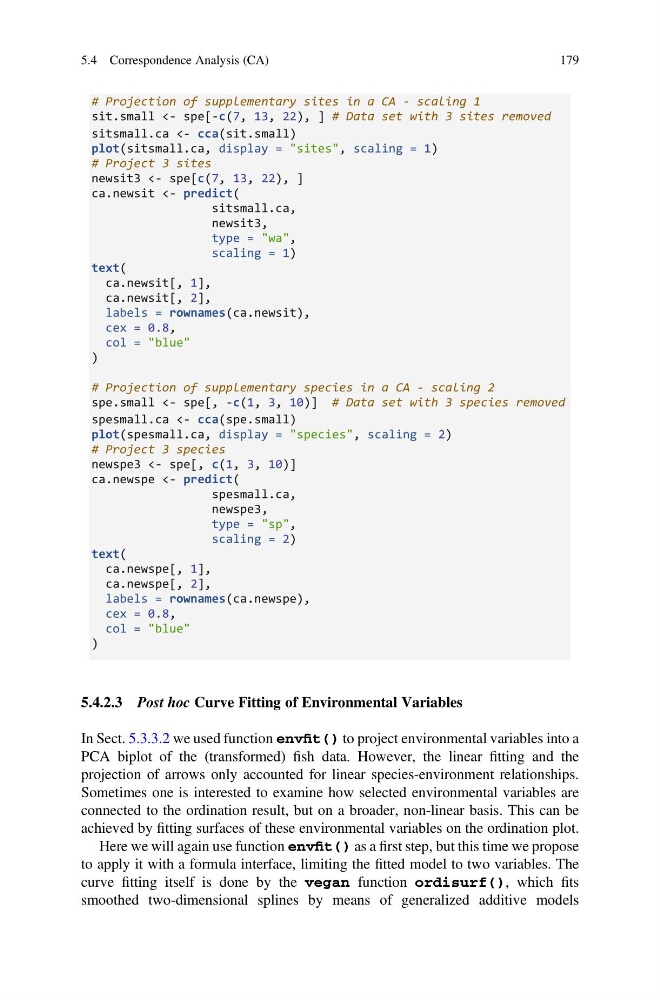
# Projection of supplementary sites in a CA - scaling 1
sit.small <- spe[-c(7, 13, 22), ] # Data set with 3 sites removed
sitsmall.ca <- cca(sit.small)
plot(sitsmall.ca, display = "sites", scaling = 1)
# Project 3 sites
newsit3 <- spe[c(7, 13, 22), ]
ca.newsit <- predict(
sitsmall.ca,
newsit3,
type = "wa",
scaling = 1)
text(
ca.newsit[, 1],
ca.newsit[, 2],
labels = rownames(ca.newsit),
cex = 0.8,
col = "blue"
)
# Projection of supplementary species in a CA - scaling 2
spe.small <- spe[, -c(1, 3, 10)] # Data set with 3 species removed
spesmall.ca <- cca(spe.small)
plot(spesmall.ca, display = "species", scaling = 2)
# Project 3 species
newspe3 <- spe[, c(1, 3, 10)]
ca.newspe <- predict(
spesmall.ca,
newspe3,
type = "sp",
scaling = 2)
text(
ca.newspe[, 1],
ca.newspe[, 2],
labels = rownames(ca.newspe),
cex = 0.8,
col = "blue"
)
5.4.2.3 Post hoc Curve Fitting of Environmental Variables
In Sect. 5.3.3.2 we used function envfit() to project environmental variables into a
PCA biplot of the (transformed) fish data. However, the linear fitting and the
projection of arrows only accounted for linear species-environment relationships.
Sometimes one is interested to examine how selected environmental variables are
connected to the ordination result, but on a broader, non-linear basis. This can be
achieved by fitting surfaces of these environmental variables on the ordination plot.
Here we will again use function envfit() as a first step, but this time we propose
to apply it with a formula interface, limiting the fitted model to two variables. The
curve fitting itself is done by the vegan function ordisurf(), which fits
smoothed two-dimensional splines by means of generalized additive models
5.4 Correspondence Analysis (CA)
179