

The first axis has a large eigenvalue. In CA, values over 0.6 indicate a very strong
gradient in the data. What proportion of the total inertia does the first axis
account for?
The eigenvalues are the same in both scalings. The scaling affects the
eigenvectors to be drawn but not the eigenvalues.
# Scree plot and broken stick model using vegan’s screeplot.cca()
screeplot(spe.ca, bstick = TRUE, npcs = length(spe.ca$CA$eig)
The first axis is extremely dominant, as can be seen from the bar plot as well as
the numerical results.
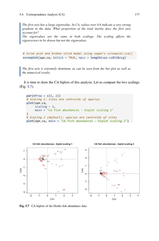
It is time to draw the CA biplots of this analysis. Let us compare the two scalings
(Fig. 5.7).
par(mfrow = c(1, 2))
# Scaling 1: sites are centroids of species
plot(spe.ca,
scaling = 1,
main = "CA fish abundances - biplot scaling 1"
)
# Scaling 2 (default): species are centroids of sites
plot(spe.ca, main = "CA fish abundances - biplot scaling 2")
-2
-1
0
1
2
3
-4
-3
-2
-1
0
1
CA fish abundances - biplot scaling 1
CA1
CA2
Cogo
Satr
Phph
Babl
Thth
Teso
Chna
Pato
Lele
Sqce
Baba
Albi
Gogo
Eslu
Pefl
Rham Legi
Scer
Cyca
Titi
Abbr
Icme
Gyce
Ruru
Blbj Alal
Anan
1
2
3
4
5
6
7
9
10
11
12
13
14
15
16
17
18
19
20
21
22
23
2425
26 27
28
29
30
- 2
- 1
0
1
2
3
4
-2
-1
0
1
2
3
CA fish abundances - biplot scaling 2
CA1
CA2
Cogo
Satr
Phph
Babl
Thth
Teso
Chna
Pato
Lele
Sqce
Baba
Albi
Gogo
Eslu
Pefl
Rham Legi
Scer
Cyca
Titi
Abbr
Icme Gyce
Ruru
Blbj Alal
Anan
1
2
3
4
5
6
7
9
10
11
12
13
14
15
16
17
18
19
20
21
22
23
2425
26
27
28
29
30
Fig. 5.7 CA biplots of the Doubs fish abundance data
5.4 Correspondence Analysis (CA)
177
gradient in the data. What proportion of the total inertia does the first axis
account for?
The eigenvalues are the same in both scalings. The scaling affects the
eigenvectors to be drawn but not the eigenvalues.
# Scree plot and broken stick model using vegan’s screeplot.cca()
screeplot(spe.ca, bstick = TRUE, npcs = length(spe.ca$CA$eig)
The first axis is extremely dominant, as can be seen from the bar plot as well as
the numerical results.
It is time to draw the CA biplots of this analysis. Let us compare the two scalings
(Fig. 5.7).
par(mfrow = c(1, 2))
# Scaling 1: sites are centroids of species
plot(spe.ca,
scaling = 1,
main = "CA fish abundances - biplot scaling 1"
)
# Scaling 2 (default): species are centroids of sites
plot(spe.ca, main = "CA fish abundances - biplot scaling 2")
-2
-1
0
1
2
3
-4
-3
-2
-1
0
1
CA fish abundances - biplot scaling 1
CA1
CA2
Cogo
Satr
Phph
Babl
Thth
Teso
Chna
Pato
Lele
Sqce
Baba
Albi
Gogo
Eslu
Pefl
Rham Legi
Scer
Cyca
Titi
Abbr
Icme
Gyce
Ruru
Blbj Alal
Anan
1
2
3
4
5
6
7
9
10
11
12
13
14
15
16
17
18
19
20
21
22
23
2425
26 27
28
29
30
- 2
- 1
0
1
2
3
4
-2
-1
0
1
2
3
CA fish abundances - biplot scaling 2
CA1
CA2
Cogo
Satr
Phph
Babl
Thth
Teso
Chna
Pato
Lele
Sqce
Baba
Albi
Gogo
Eslu
Pefl
Rham Legi
Scer
Cyca
Titi
Abbr
Icme Gyce
Ruru
Blbj Alal
Anan
1
2
3
4
5
6
7
9
10
11
12
13
14
15
16
17
18
19
20
21
22
23
2425
26
27
28
29
30
Fig. 5.7 CA biplots of the Doubs fish abundance data
5.4 Correspondence Analysis (CA)
177