

close to the point representing an object is more likely to be found in that object,
or to have a higher frequency there than in objects that are further away in the
joint plot.
The broken stick model, explained in Sect. 5.3.2.3, can be applied to CA axes for
guidance as to the number of axes to retain. Our application below will concern the
raw fish abundance data.
5.4.2 CA Using Function cca() of Package vegan
5.4.2.1 Running the Analysis and Drawing the Biplots
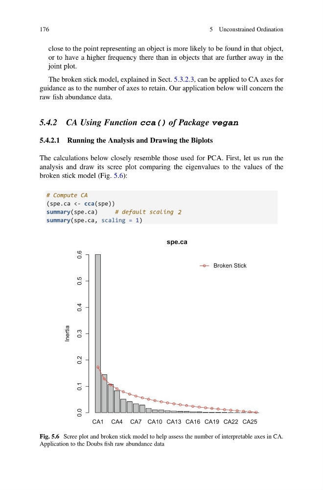
The calculations below closely resemble those used for PCA. First, let us run the
analysis and draw its scree plot comparing the eigenvalues to the values of the
broken stick model (Fig. 5.6):
# Compute CA
(spe.ca <- cca(spe))
summary(spe.ca)
# default scaling 2
summary(spe.ca, scaling = 1)
CA1 CA4 CA7 CA10 CA13 CA16 CA19 CA22 CA25
spe.ca
Inertia
0.0
0.1
0.2
0.3
0.4
0.5
0.6
Broken Stick
Fig. 5.6 Scree plot and broken stick model to help assess the number of interpretable axes in CA.
Application to the Doubs fish raw abundance data
176
5 Unconstrained Ordination
or to have a higher frequency there than in objects that are further away in the
joint plot.
The broken stick model, explained in Sect. 5.3.2.3, can be applied to CA axes for
guidance as to the number of axes to retain. Our application below will concern the
raw fish abundance data.
5.4.2 CA Using Function cca() of Package vegan
5.4.2.1 Running the Analysis and Drawing the Biplots
The calculations below closely resemble those used for PCA. First, let us run the
analysis and draw its scree plot comparing the eigenvalues to the values of the
broken stick model (Fig. 5.6):
# Compute CA
(spe.ca <- cca(spe))
summary(spe.ca)
# default scaling 2
summary(spe.ca, scaling = 1)
CA1 CA4 CA7 CA10 CA13 CA16 CA19 CA22 CA25
spe.ca
Inertia
0.0
0.1
0.2
0.3
0.4
0.5
0.6
Broken Stick
Fig. 5.6 Scree plot and broken stick model to help assess the number of interpretable axes in CA.
Application to the Doubs fish raw abundance data
176
5 Unconstrained Ordination