

# Combining clustering and ordination results
# Clustering the objects using the environmental data: Euclidean
# distance after standardizing the variables, followed by Ward
# clustering
env.w <- hclust(dist(scale(env)), "ward.D")
# Cut the dendrogram to yield 4 groups
gr <- cutree(env.w, k = 4)
grl <- levels(factor(gr))
# Extract the site scores, scaling 1
sit.sc1 <- scores(env.pca, display = "wa", scaling = 1)
# Plot the sites with cluster symbols and colours (scaling 1)
p <- plot(
env.pca,
display = "wa",
scaling = 1,
type = "n",
main = "PCA correlation + clusters"
)
-1.0
-0.5
0.0
0.5
1.0
1.5
-1.0
-0.5
0.0
0.5
1.0
PCA correlation + clusters
PC1
PC2
1
2
3
4
5
6
7
9
10
11
12
13 14
15
16
17
18
19 20
21
22
23
24
25
26
27
28
29
30
Cluster 1
Cluster 2
Cluster 3
Cluster 4
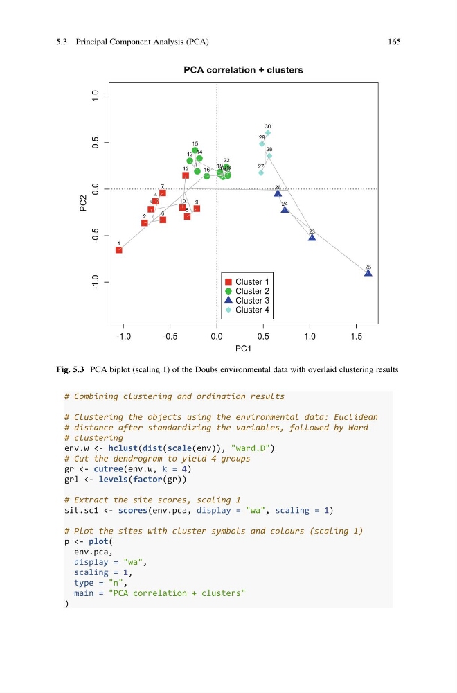
Fig. 5.3 PCA biplot (scaling 1) of the Doubs environmental data with overlaid clustering results
5.3 Principal Component Analysis (PCA)
165
# Clustering the objects using the environmental data: Euclidean
# distance after standardizing the variables, followed by Ward
# clustering
env.w <- hclust(dist(scale(env)), "ward.D")
# Cut the dendrogram to yield 4 groups
gr <- cutree(env.w, k = 4)
grl <- levels(factor(gr))
# Extract the site scores, scaling 1
sit.sc1 <- scores(env.pca, display = "wa", scaling = 1)
# Plot the sites with cluster symbols and colours (scaling 1)
p <- plot(
env.pca,
display = "wa",
scaling = 1,
type = "n",
main = "PCA correlation + clusters"
)
-1.0
-0.5
0.0
0.5
1.0
1.5
-1.0
-0.5
0.0
0.5
1.0
PCA correlation + clusters
PC1
PC2
1
2
3
4
5
6
7
9
10
11
12
13 14
15
16
17
18
19 20
21
22
23
24
25
26
27
28
29
30
Cluster 1
Cluster 2
Cluster 3
Cluster 4
Fig. 5.3 PCA biplot (scaling 1) of the Doubs environmental data with overlaid clustering results
5.3 Principal Component Analysis (PCA)
165