

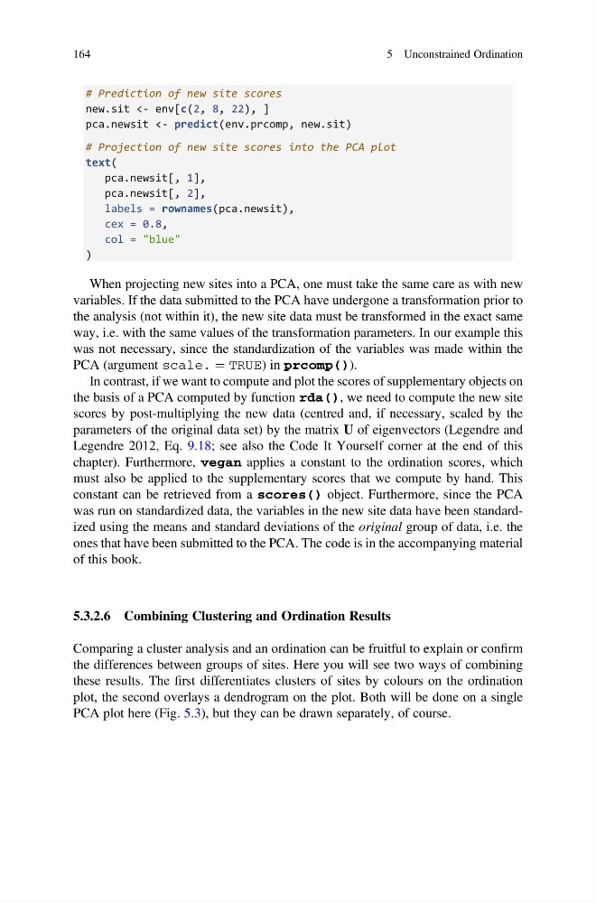
# Prediction of new site scores
new.sit <- env[c(2, 8, 22), ]
pca.newsit <- predict(env.prcomp, new.sit)
# Projection of new site scores into the PCA plot
text(
pca.newsit[, 1],
pca.newsit[, 2],
labels = rownames(pca.newsit),
cex = 0.8,
col = "blue"
)
When projecting new sites into a PCA, one must take the same care as with new
variables. If the data submitted to the PCA have undergone a transformation prior to
the analysis (not within it), the new site data must be transformed in the exact same
way, i.e. with the same values of the transformation parameters. In our example this
was not necessary, since the standardization of the variables was made within the
PCA (argument scale. ¼ TRUE) in prcomp()).
In contrast, if we want to compute and plot the scores of supplementary objects on
the basis of a PCA computed by function rda(), we need to compute the new site
scores by post-multiplying the new data (centred and, if necessary, scaled by the
parameters of the original data set) by the matrix U of eigenvectors (Legendre and
Legendre 2012, Eq. 9.18; see also the Code It Yourself corner at the end of this
chapter). Furthermore, vegan applies a constant to the ordination scores, which
must also be applied to the supplementary scores that we compute by hand. This
constant can be retrieved from a scores() object. Furthermore, since the PCA
was run on standardized data, the variables in the new site data have been standardized using the means and standard deviations of the original group of data, i.e. the
ones that have been submitted to the PCA. The code is in the accompanying material
of this book.
5.3.2.6 Combining Clustering and Ordination Results
Comparing a cluster analysis and an ordination can be fruitful to explain or confirm
the differences between groups of sites. Here you will see two ways of combining
these results. The first differentiates clusters of sites by colours on the ordination
plot, the second overlays a dendrogram on the plot. Both will be done on a single
PCA plot here (Fig. 5.3), but they can be drawn separately, of course.
164
5 Unconstrained Ordination
new.sit <- env[c(2, 8, 22), ]
pca.newsit <- predict(env.prcomp, new.sit)
# Projection of new site scores into the PCA plot
text(
pca.newsit[, 1],
pca.newsit[, 2],
labels = rownames(pca.newsit),
cex = 0.8,
col = "blue"
)
When projecting new sites into a PCA, one must take the same care as with new
variables. If the data submitted to the PCA have undergone a transformation prior to
the analysis (not within it), the new site data must be transformed in the exact same
way, i.e. with the same values of the transformation parameters. In our example this
was not necessary, since the standardization of the variables was made within the
PCA (argument scale. ¼ TRUE) in prcomp()).
In contrast, if we want to compute and plot the scores of supplementary objects on
the basis of a PCA computed by function rda(), we need to compute the new site
scores by post-multiplying the new data (centred and, if necessary, scaled by the
parameters of the original data set) by the matrix U of eigenvectors (Legendre and
Legendre 2012, Eq. 9.18; see also the Code It Yourself corner at the end of this
chapter). Furthermore, vegan applies a constant to the ordination scores, which
must also be applied to the supplementary scores that we compute by hand. This
constant can be retrieved from a scores() object. Furthermore, since the PCA
was run on standardized data, the variables in the new site data have been standardized using the means and standard deviations of the original group of data, i.e. the
ones that have been submitted to the PCA. The code is in the accompanying material
of this book.
5.3.2.6 Combining Clustering and Ordination Results
Comparing a cluster analysis and an ordination can be fruitful to explain or confirm
the differences between groups of sites. Here you will see two ways of combining
these results. The first differentiates clusters of sites by colours on the ordination
plot, the second overlays a dendrogram on the plot. Both will be done on a single
PCA plot here (Fig. 5.3), but they can be drawn separately, of course.
164
5 Unconstrained Ordination