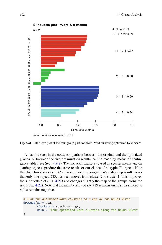
As can be seen in the code, comparison between the original and the optimized
groups, or between the two optimization results, can be made by means of contingency tables (see Sect. 4.9.2). The two optimizations (based on species means and on
starting objects) produce the same result for our choice of 4 “typical” objects. Note
that this choice is critical. Comparison with the original Ward 4-group result shows
that only one object, #15, has been moved from cluster 2 to cluster 1. This improves
the silhouette plot (Fig. 4.21) and changes slightly the map of the groups along the
river (Fig. 4.22). Note that the membership of site #19 remains unclear: its silhouette
value remains negative.
# Plot the optimized Ward clusters on a map of the Doubs River
drawmap(xy = spa,
clusters = spech.ward.gk,
main = "Four optimized Ward clusters along the Doubs River"
)
25
24
23
20
26
30
29
28
27
21
22
19
5
9
16
18
17
15
10
6
1
4
14
13
11
7
3
12
2
Silhouette width s i
0.0
0.2
0.4
0.6
0.8
1.0
Silhouette plot - Ward & k-means
Average silhouette width : 0.37
n = 29
4 clusters C j
j : n j | ave i Cj s i
1 : 12 | 0.37
2 : 6 | 0.08
3 : 8 | 0.59
4 : 3 | 0.34
Fig. 4.21 Silhouette plot of the four-group partition from Ward clustering optimized by k-means
102
4 Cluster Analysis