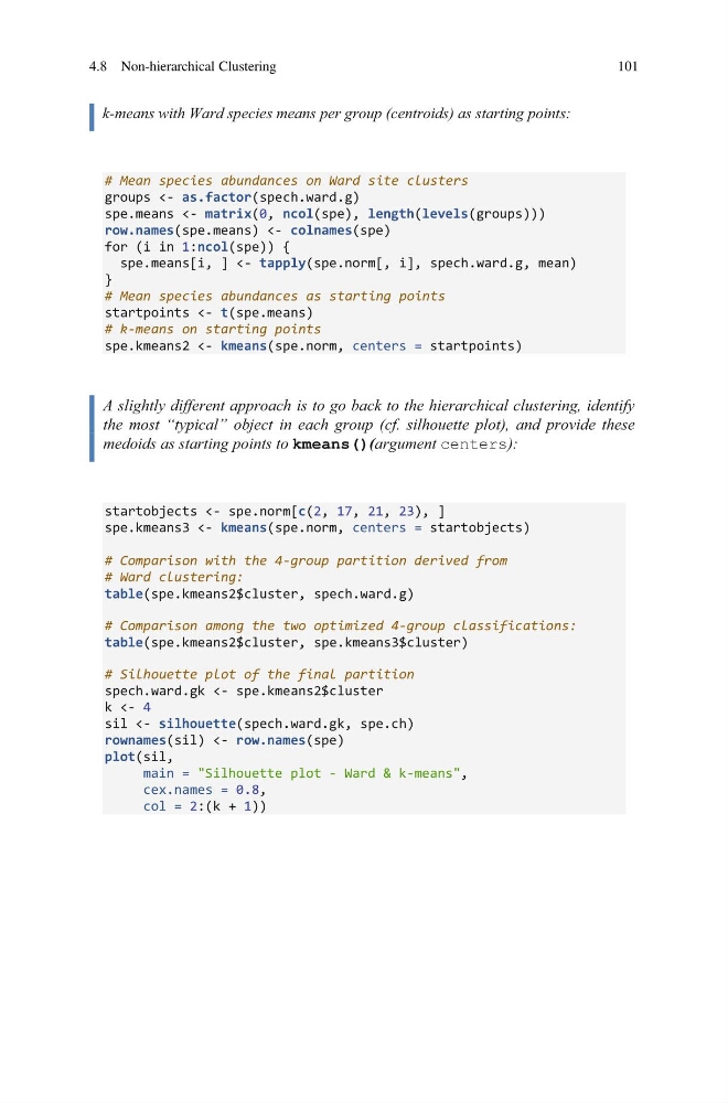
k-means with Ward species means per group (centroids) as starting points:
# Mean species abundances on Ward site clusters
groups <- as.factor(spech.ward.g)
spe.means <- matrix(0, ncol(spe), length(levels(groups)))
row.names(spe.means) <- colnames(spe)
for (i in 1:ncol(spe)) {
spe.means[i, ] <- tapply(spe.norm[, i], spech.ward.g, mean)
}
# Mean species abundances as starting points
startpoints <- t(spe.means)
# k-means on starting points
spe.kmeans2 <- kmeans(spe.norm, centers = startpoints)
A slightly different approach is to go back to the hierarchical clustering, identify
the most “typical” object in each group (cf. silhouette plot), and provide these
medoids as starting points to kmeans()(argument centers):
startobjects <- spe.norm[c(2, 17, 21, 23), ]
spe.kmeans3 <- kmeans(spe.norm, centers = startobjects)
# Comparison with the 4-group partition derived from
# Ward clustering:
table(spe.kmeans2$cluster, spech.ward.g)
# Comparison among the two optimized 4-group classifications:
table(spe.kmeans2$cluster, spe.kmeans3$cluster)
# Silhouette plot of the final partition
spech.ward.gk <- spe.kmeans2$cluster
k <- 4
sil <- silhouette(spech.ward.gk, spe.ch)
rownames(sil) <- row.names(spe)
plot(sil,
main = "Silhouette plot - Ward & k-means",
cex.names = 0.8,
col = 2:(k + 1))
4.8 Non-hierarchical Clustering
101