

# Choose the number of clusters
k <- 4
# Silhouette plot of the final partition
spech.ward.g <- cutree(spe.ch.ward, k = k)
sil <- silhouette(spech.ward.g, spe.ch)
rownames(sil) <- row.names(spe)
plot(
sil,
main = "Silhouette plot - Chord - Ward",
cex.names = 0.8,
col = 2:(k + 1),
nmax = 100
)
25
24
23
20
26
30
28
29
27
22
21
15
19
5
18
9
16
17
10
6
1
14
4
13
11
7
12
3
2
Silhouette width s i
0.0
0.2
0.4
0.6
0.8
1.0
Silhouette plot - Chord - Ward
Average silhouette width : 0.35
n = 29
4 clusters C j
j : n j | ave i Cj s i
1 : 11 | 0.37
2 : 7 | 0.04
3 : 8 | 0.60
4 : 3 | 0.34
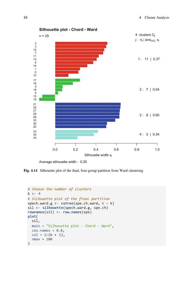
Fig. 4.14 Silhouette plot of the final, four-group partition from Ward clustering
88
4 Cluster Analysis
k <- 4
# Silhouette plot of the final partition
spech.ward.g <- cutree(spe.ch.ward, k = k)
sil <- silhouette(spech.ward.g, spe.ch)
rownames(sil) <- row.names(spe)
plot(
sil,
main = "Silhouette plot - Chord - Ward",
cex.names = 0.8,
col = 2:(k + 1),
nmax = 100
)
25
24
23
20
26
30
28
29
27
22
21
15
19
5
18
9
16
17
10
6
1
14
4
13
11
7
12
3
2
Silhouette width s i
0.0
0.2
0.4
0.6
0.8
1.0
Silhouette plot - Chord - Ward
Average silhouette width : 0.35
n = 29
4 clusters C j
j : n j | ave i Cj s i
1 : 11 | 0.37
2 : 7 | 0.04
3 : 8 | 0.60
4 : 3 | 0.34
Fig. 4.14 Silhouette plot of the final, four-group partition from Ward clustering
88
4 Cluster Analysis