

46
S.M.P . Benbow
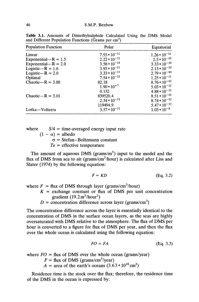
Table 3.1. Amounts of Dimethylsulphide Calculated Using the DMS Model
and Different Population Functions (Grams per crrr')
Population Function
Polar
Equatorial
Linear
Exponential-R = 1.5
Exponential-R = 2.0
Logistic-R = 1.6
Logistic-R = 2.0
Optimal
Chaotic-R = 3.00
Chaotic-R = 3.01
Lotka-Volterra
7.55 * 1011
2.22* 1011
3.58 * 1011
3.95 * 1011
3.33 * 1011
7.54*10- 11
82.18
1.90* 10+
7
0.132
839520.4
2.34* 1011
119494.9
3.57 *1011
1.26* 1011
2.5 * 1010
3.33 * 1010
2.13 * 10- 10
2.79* 10- 10
1.25 * 1011
8.76* 1012
5.03 * 10- 12
4.88 *10- 12
8.51 * 10- 12
8.74 * 1012
5.47 * 10- 12
1.03* 10- 8
where
5/4 = time-averaged energy input rate
(1 - a) = albedo
cr = Stefan- Boltzmann constant
Te = effective temperature
The amount of aqueous DMS (grams/m") input to the model and the
flux of DMS from sea to air (grams/cnr'zhour) is calculated after Liss and
Slater (1974) by the following equation:
F= KD
(Eq .3.2)
where F = flux of DMS through layer (grams/cnr'zhour)
K = exchange constant or flux of DMS per unit concentration
gradient (19.2m
3/hour1 )
D = concentration difference across layer (grams/em")
The concentration difference across the layer is essentially identical to the
concentration of DMS in the surface ocean layers, as the seas are highly
oversaturated with DMS relative to the atmosphere. The flux of DMS per
hour is converted to a figure for flux of DMS per year, and then the flux
over the whole ocean is calculated using the following equation:
FO=FA
(Eq .3.3)
where FO = flux of DMS over the whole ocean (grams/year)
F = flux of DMS (grams/emf/year)
A = area of the earth's oceans (3.63 *10
18 em")
Residence time is the stock over the flux; therefore, the residence time
of the DMS in the ocean is expressed by:
S.M.P . Benbow
Table 3.1. Amounts of Dimethylsulphide Calculated Using the DMS Model
and Different Population Functions (Grams per crrr')
Population Function
Polar
Equatorial
Linear
Exponential-R = 1.5
Exponential-R = 2.0
Logistic-R = 1.6
Logistic-R = 2.0
Optimal
Chaotic-R = 3.00
Chaotic-R = 3.01
Lotka-Volterra
7.55 * 1011
2.22* 1011
3.58 * 1011
3.95 * 1011
3.33 * 1011
7.54*10- 11
82.18
1.90* 10+
7
0.132
839520.4
2.34* 1011
119494.9
3.57 *1011
1.26* 1011
2.5 * 1010
3.33 * 1010
2.13 * 10- 10
2.79* 10- 10
1.25 * 1011
8.76* 1012
5.03 * 10- 12
4.88 *10- 12
8.51 * 10- 12
8.74 * 1012
5.47 * 10- 12
1.03* 10- 8
where
5/4 = time-averaged energy input rate
(1 - a) = albedo
cr = Stefan- Boltzmann constant
Te = effective temperature
The amount of aqueous DMS (grams/m") input to the model and the
flux of DMS from sea to air (grams/cnr'zhour) is calculated after Liss and
Slater (1974) by the following equation:
F= KD
(Eq .3.2)
where F = flux of DMS through layer (grams/cnr'zhour)
K = exchange constant or flux of DMS per unit concentration
gradient (19.2m
3/hour1 )
D = concentration difference across layer (grams/em")
The concentration difference across the layer is essentially identical to the
concentration of DMS in the surface ocean layers, as the seas are highly
oversaturated with DMS relative to the atmosphere. The flux of DMS per
hour is converted to a figure for flux of DMS per year, and then the flux
over the whole ocean is calculated using the following equation:
FO=FA
(Eq .3.3)
where FO = flux of DMS over the whole ocean (grams/year)
F = flux of DMS (grams/emf/year)
A = area of the earth's oceans (3.63 *10
18 em")
Residence time is the stock over the flux; therefore, the residence time
of the DMS in the ocean is expressed by: