

156
in the air and water. Strictly speaking, the air–water CO 2 flux should be calculated
from the fugacity of CO 2 (fCO 2 ), which is the partial pressure of an ideal gas with
the same chemical potential as the real gas. However, for the sake of simplicity no
distinction between pCO 2 and fCO 2 has been made in this chapter. The difference in
the estimated CO 2 fluxes would be very small (Weiss 1974).
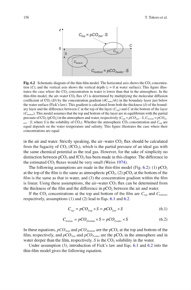
The following assumptions are made in the thin-film model (Fig. 6.2): (1) pCO 2
at the top of the film is the same as atmospheric pCO 2 , (2) pCO 2 at the bottom of the
film is the same as that in water, and (3) the concentration gradient within the film
is linear. Using these assumptions, the air–water CO 2 flux can be determined from
the thickness of the film and the difference in pCO 2 between the air and water.
If the CO 2 concentrations at the top and bottom of the film are C top and C bottom ,
respectively, assumptions (1) and (2) lead to Eqs. 6.1 and 6.2.
C
pCO
S pCO
S
top
t op
air
=
´ =
´
2
2
(6.1)
C
pCO
S pCO
S
bottom
bottom
w ater
=
´ =
´
2
2
(6.2)
In these equations, pCO 2top and pCO 2bottom are the pCO 2 at the top and bottom of the
film, respectively, and pCO 2air and pCO 2water are the pCO 2 in the atmosphere and in
water deeper than the film, respectively. S is the CO 2 solubility in the water.
Under assumption (3), introduction of Fick’s law and Eqs. 6.1 and 6.2 into the
thin-film model gives the following equation.
C
z
C top = pCO 2air . S
C top
C bottom
δ
C bottom = pCO 2water . S
0
Fig. 6.2 Schematic diagram of the thin-film model. The horizontal axis shows the CO 2 concentration (C), and the vertical axis shows the vertical depth (z = 0 at water surface). This figure illustrates the case where the CO 2 concentration in water is lower than that in the atmosphere. In the
thin-film model, the air–water CO 2 flux (F) is determined by multiplying the molecular diffusion
coefficient of CO 2 (D) by the concentration gradient (∂C water /∂z) in the boundary layer just below
the water surface (Fick’s law). This gradient is calculated from both the thickness (δ) of the boundary layer and the difference between C at the top of the layer (C top ) and C at the bottom of the layer
(C bottom ). This model assumes that the top and bottom of the layer are in equilibrium with the partial
pressure of CO 2 (pCO 2 ) in the atmosphere and water, respectively (C top = pCO 2air · S, C bottom = pCO 2water · S; where S is the solubility of CO 2 ). Whether the atmospheric CO 2 concentration and C top are
equal depends on the water temperature and salinity. This figure illustrates the case where their
concentrations are equal
T. Tokoro et al.
in the air and water. Strictly speaking, the air–water CO 2 flux should be calculated
from the fugacity of CO 2 (fCO 2 ), which is the partial pressure of an ideal gas with
the same chemical potential as the real gas. However, for the sake of simplicity no
distinction between pCO 2 and fCO 2 has been made in this chapter. The difference in
the estimated CO 2 fluxes would be very small (Weiss 1974).
The following assumptions are made in the thin-film model (Fig. 6.2): (1) pCO 2
at the top of the film is the same as atmospheric pCO 2 , (2) pCO 2 at the bottom of the
film is the same as that in water, and (3) the concentration gradient within the film
is linear. Using these assumptions, the air–water CO 2 flux can be determined from
the thickness of the film and the difference in pCO 2 between the air and water.
If the CO 2 concentrations at the top and bottom of the film are C top and C bottom ,
respectively, assumptions (1) and (2) lead to Eqs. 6.1 and 6.2.
C
pCO
S pCO
S
top
t op
air
=
´ =
´
2
2
(6.1)
C
pCO
S pCO
S
bottom
bottom
w ater
=
´ =
´
2
2
(6.2)
In these equations, pCO 2top and pCO 2bottom are the pCO 2 at the top and bottom of the
film, respectively, and pCO 2air and pCO 2water are the pCO 2 in the atmosphere and in
water deeper than the film, respectively. S is the CO 2 solubility in the water.
Under assumption (3), introduction of Fick’s law and Eqs. 6.1 and 6.2 into the
thin-film model gives the following equation.
C
z
C top = pCO 2air . S
C top
C bottom
δ
C bottom = pCO 2water . S
0
Fig. 6.2 Schematic diagram of the thin-film model. The horizontal axis shows the CO 2 concentration (C), and the vertical axis shows the vertical depth (z = 0 at water surface). This figure illustrates the case where the CO 2 concentration in water is lower than that in the atmosphere. In the
thin-film model, the air–water CO 2 flux (F) is determined by multiplying the molecular diffusion
coefficient of CO 2 (D) by the concentration gradient (∂C water /∂z) in the boundary layer just below
the water surface (Fick’s law). This gradient is calculated from both the thickness (δ) of the boundary layer and the difference between C at the top of the layer (C top ) and C at the bottom of the layer
(C bottom ). This model assumes that the top and bottom of the layer are in equilibrium with the partial
pressure of CO 2 (pCO 2 ) in the atmosphere and water, respectively (C top = pCO 2air · S, C bottom = pCO 2water · S; where S is the solubility of CO 2 ). Whether the atmospheric CO 2 concentration and C top are
equal depends on the water temperature and salinity. This figure illustrates the case where their
concentrations are equal
T. Tokoro et al.