

25. Ecosystem Modeling
commodities used in ecosystem models. Initially,
models were univariate (they considered the transfer of energy or nutrients but not both), but over
time, multiple commodity models have become
more prevalent.
Modeling Phase
There is a myriad of different mathematical approaches that have been applied to the formulation
of ecological models. However, two related mathematical formulations are most often used to predict
the change in the state variables of a system. In the
first, the difference equation, the change in the state
variable at a given time t (denoted Ax t ) over a fixed
interval of time (M) is used to compute the new
value of the state variable at the next time t + I1t
(denoted Xt+ LlJ The resultant equations are of the
form:
X t + Llt = X t + Axt or Axt = Xt+Llt - Xt (25.1)
The emphasis is on the quantitative value on the
condition or state of each of the parts and on determining how these states change over time. The
change in the quantitative measure of the parts is
as change in a state variable represented by such an
equation. This will be made more explicit in the
examples that follow.
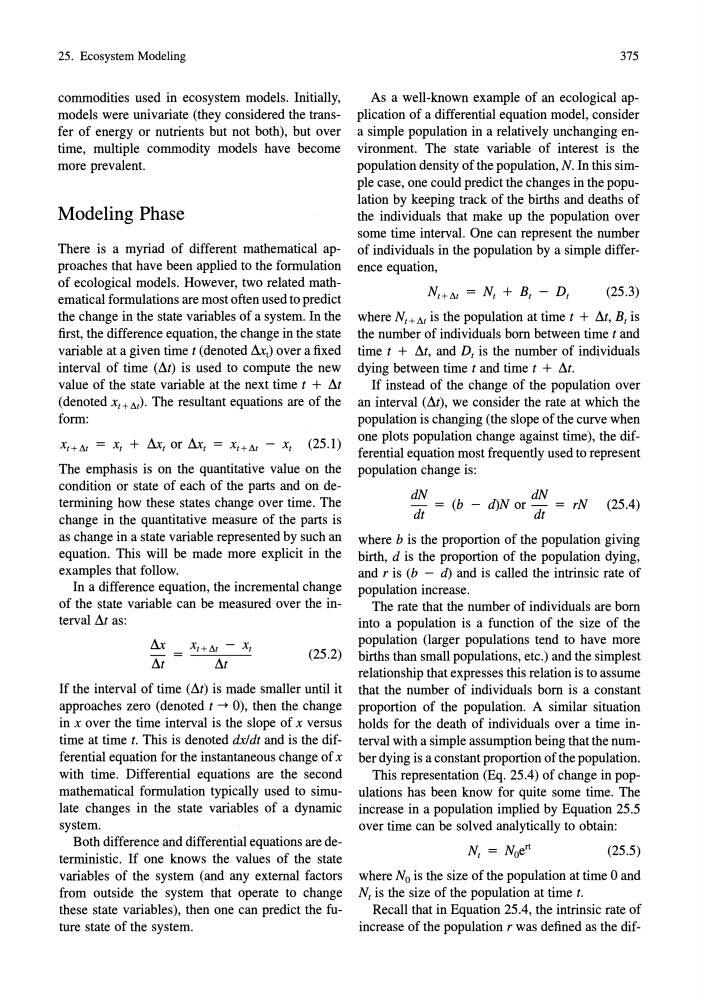
In a difference equation, the incremental change
of the state variable can be measured over the intervall1t as:
(25.2)
If the interval of time (M) is made smaller until it
approaches zero (denoted t ~ 0), then the change
in x over the time interval is the slope of x versus
time at time t. This is denoted dx/dt and is the differential equation for the instantaneous change of x
with time. Differential equations are the second
mathematical formulation typically used to simulate changes in the state variables of a dynamic
system.
Both difference and differential equations are deterministic. If one knows the values of the state
variables of the system (and any external factors
from outside the system that operate to change
these state variables), then one can predict the future state of the system.
375
As a well-known example of an ecological application of a differential equation model, consider
a simple population in a relatively unchanging environment. The state variable of interest is the
population density of the population, N. In this simple case, one could predict the changes in the population by keeping track of the births and deaths of
the individuals that make up the population over
some time interval. One can represent the number
of individuals in the population by a simple difference equation,
(25.3)
where NtHt is the popUlation at time t + I1t, Bt is
the number of individuals born between time t and
time t + M, and Dt is the number of individuals
dying between time t and time t + I1t.
If instead of the change of the popUlation over
an interval (I1t), we consider the rate at which the
population is changing (the slope of the curve when
one plots population change against time), the differential equation most frequently used to represent
population change is:
dN
dN
dt = (b - d)N or dt = rN (25.4)
where b is the proportion of the population giving
birth, d is the proportion of the popUlation dying,
and r is (b - d) and is called the intrinsic rate of
population increase.
The rate that the number of individuals are born
into a population is a function of the size of the
population (larger populations tend to have more
births than small populations, etc.) and the simplest
relationship that expresses this relation is to assume
that the number of individuals born is a constant
proportion of the population. A similar situation
holds for the death of individuals over a time interval with a simple assumption being that the number dying is a constant proportion of the popUlation.
This representation (Eq. 25.4) of change in populations has been know for quite some time. The
increase in a population implied by Equation 25.5
over time can be solved analytically to obtain:
(25.5)
where No is the size of the population at time 0 and
Nt is the size of the population at time t.
Recall that in Equation 25.4, the intrinsic rate of
increase of the population r was defined as the dif-
commodities used in ecosystem models. Initially,
models were univariate (they considered the transfer of energy or nutrients but not both), but over
time, multiple commodity models have become
more prevalent.
Modeling Phase
There is a myriad of different mathematical approaches that have been applied to the formulation
of ecological models. However, two related mathematical formulations are most often used to predict
the change in the state variables of a system. In the
first, the difference equation, the change in the state
variable at a given time t (denoted Ax t ) over a fixed
interval of time (M) is used to compute the new
value of the state variable at the next time t + I1t
(denoted Xt+ LlJ The resultant equations are of the
form:
X t + Llt = X t + Axt or Axt = Xt+Llt - Xt (25.1)
The emphasis is on the quantitative value on the
condition or state of each of the parts and on determining how these states change over time. The
change in the quantitative measure of the parts is
as change in a state variable represented by such an
equation. This will be made more explicit in the
examples that follow.
In a difference equation, the incremental change
of the state variable can be measured over the intervall1t as:
(25.2)
If the interval of time (M) is made smaller until it
approaches zero (denoted t ~ 0), then the change
in x over the time interval is the slope of x versus
time at time t. This is denoted dx/dt and is the differential equation for the instantaneous change of x
with time. Differential equations are the second
mathematical formulation typically used to simulate changes in the state variables of a dynamic
system.
Both difference and differential equations are deterministic. If one knows the values of the state
variables of the system (and any external factors
from outside the system that operate to change
these state variables), then one can predict the future state of the system.
375
As a well-known example of an ecological application of a differential equation model, consider
a simple population in a relatively unchanging environment. The state variable of interest is the
population density of the population, N. In this simple case, one could predict the changes in the population by keeping track of the births and deaths of
the individuals that make up the population over
some time interval. One can represent the number
of individuals in the population by a simple difference equation,
(25.3)
where NtHt is the popUlation at time t + I1t, Bt is
the number of individuals born between time t and
time t + M, and Dt is the number of individuals
dying between time t and time t + I1t.
If instead of the change of the popUlation over
an interval (I1t), we consider the rate at which the
population is changing (the slope of the curve when
one plots population change against time), the differential equation most frequently used to represent
population change is:
dN
dN
dt = (b - d)N or dt = rN (25.4)
where b is the proportion of the population giving
birth, d is the proportion of the popUlation dying,
and r is (b - d) and is called the intrinsic rate of
population increase.
The rate that the number of individuals are born
into a population is a function of the size of the
population (larger populations tend to have more
births than small populations, etc.) and the simplest
relationship that expresses this relation is to assume
that the number of individuals born is a constant
proportion of the population. A similar situation
holds for the death of individuals over a time interval with a simple assumption being that the number dying is a constant proportion of the popUlation.
This representation (Eq. 25.4) of change in populations has been know for quite some time. The
increase in a population implied by Equation 25.5
over time can be solved analytically to obtain:
(25.5)
where No is the size of the population at time 0 and
Nt is the size of the population at time t.
Recall that in Equation 25.4, the intrinsic rate of
increase of the population r was defined as the dif-