

172
steady state condition requirement under field conditions. To avoid undesirable effects, typically from
the diurnal variation in important micrometeorological variables (e.g., solar radiation, air temperature, humidity), it is generally accepted that a 30minute sampling interval is adequate to achieve an
overall accuracy of about 10%, in near-neutral conditions (Lenschow et al. 1994; Baldocchi et al.
1988; Verma 1990). Longer averaging times to
measure covariance are generally not suggested.
It is not possible to create an eddy covariance
system that has no effect whatsoever on the fluxes
it is designed to measure. Instruments do not have
an infinitesimally small response time, nor can
nearly co-located instruments sample exactly the
same parcel of air simultaneously. As for actually
digitizing and recording the signal, the sampling
frequency and time constraints of analog or digital
filters also influence the magnitude of the loss of
signal. In this section, we describe the errors introduced into flux measurements by the components
of a typical closed-path system as described by
Moncrieff et al. (1997). The corrections that need
to be applied are frequency-dependent, that is, they
depend on the spectra and co-spectra shapes. ' TYPically, a small fraction of the total flux may be carried by small, high-frequency eddies that cannot be
detected by the measuring system. The approach
used here is to ascribe this "flux loss" to its component origins by a series of transfer functions. A
transfer function is simply a multiplier in the range
o to 1 that varies with frequency. Moore (1986)
proposed a scheme whereby a series of transfer
functions could be defined for each of the correction terms required in an eddy covariance system.
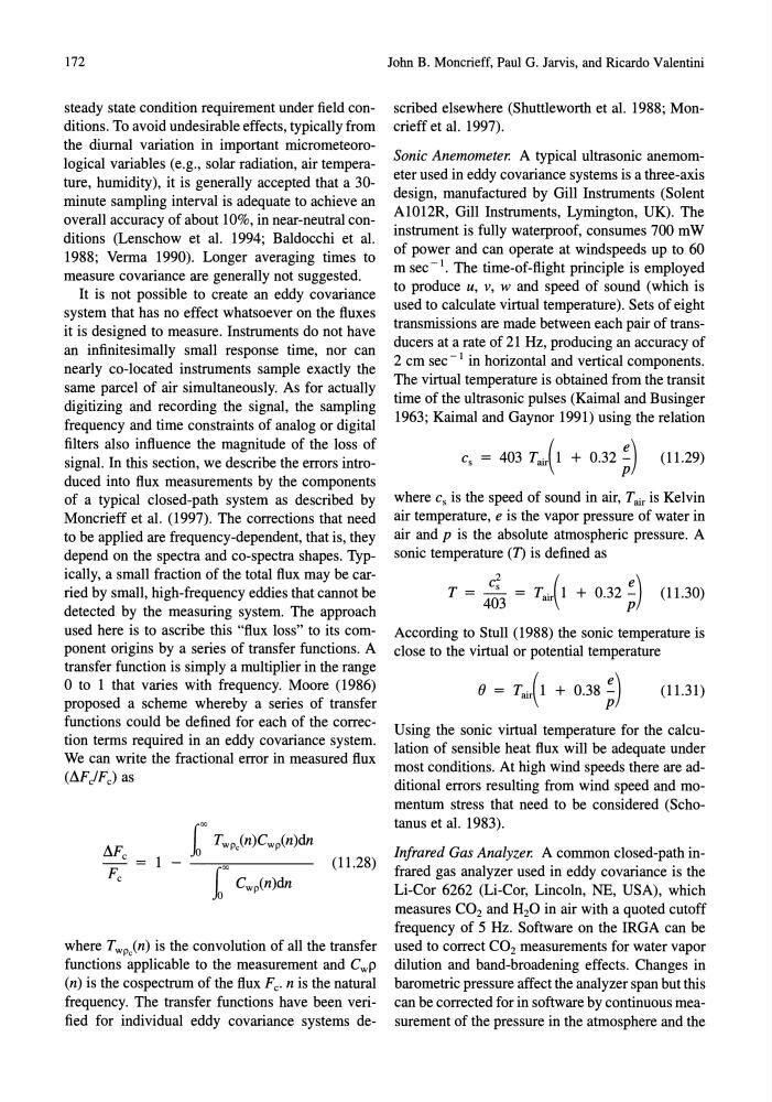
We can write the fractional error in measured flux
(MjFe) as
where Twpc(n) is the convolution of all the transfer
functions applicable to the measurement and CwP
(n) is the cospectrum of the flux Fe. n is the natural
frequency. The transfer functions have been verified for individual eddy covariance systems deJohn B. Moncrieff, Paul G. Jarvis, and Ricardo Valentini
scribed elsewhere (Shuttleworth et al. 1988; Moncrieff et al. 1997).
Sonic Anemometer. A typical ultrasonic anemometer used in eddy covariance systems is a three-axis
design, manufactured by Gill Instruments (Solent
A1012R, Gill Instruments, Lymington, UK). The
instrument is fully waterproof, consumes 700 m W
of power and can operate at windspeeds up to 60
m sec -1. The time-of-flight principle is employed
to produce u, v, w and speed of sound (which is
used to calculate virtual temperature). Sets of eight
transmissions are made between each pair of transducers at a rate of 21 Hz, producing an accuracy of
2 cm sec - 1 in horizontal and vertical components.
The virtual temperature is obtained from the transit
time of the ultrasonic pulses (Kaimal and Businger
1963; Kaimal and Gaynor 1991) using the relation
cs = 403 T air( 1 + 0.32 ~) (11.29)
where C s is the speed of sound in air, T air is Kelvin
air temperature, e is the vapor pressure of water in
air and p is the absolute atmospheric pressure. A
sonic temperature (n is defined as
T = -=L = T· (1 + 032 :)
403
atr
•
p
(11.30)
According to Stull (1988) the sonic temperature is
close to the virtual or potential temperature
(11.31)
Using the sonic virtual temperature for the calculation of sensible heat flux will be adequate under
most conditions. At high wind speeds there are additional errors resulting from wind speed and momentum stress that need to be considered (Schotanus et al. 1983).
Infrared Gas Analyzer. A common closed-path infrared gas analyzer used in eddy covariance is the
Li-Cor 6262 (Li-Cor, Lincoln, NE, USA), which
measures CO 2 and H 2 0 in air with a quoted cutoff
frequency of 5 Hz. Software on the IRGA can be
used to correct CO 2 measurements for water vapor
dilution and band-broadening effects. Changes in
barometric pressure affect the analyzer span but this
can be corrected for in software by continuous measurement of the pressure in the atmosphere and the
steady state condition requirement under field conditions. To avoid undesirable effects, typically from
the diurnal variation in important micrometeorological variables (e.g., solar radiation, air temperature, humidity), it is generally accepted that a 30minute sampling interval is adequate to achieve an
overall accuracy of about 10%, in near-neutral conditions (Lenschow et al. 1994; Baldocchi et al.
1988; Verma 1990). Longer averaging times to
measure covariance are generally not suggested.
It is not possible to create an eddy covariance
system that has no effect whatsoever on the fluxes
it is designed to measure. Instruments do not have
an infinitesimally small response time, nor can
nearly co-located instruments sample exactly the
same parcel of air simultaneously. As for actually
digitizing and recording the signal, the sampling
frequency and time constraints of analog or digital
filters also influence the magnitude of the loss of
signal. In this section, we describe the errors introduced into flux measurements by the components
of a typical closed-path system as described by
Moncrieff et al. (1997). The corrections that need
to be applied are frequency-dependent, that is, they
depend on the spectra and co-spectra shapes. ' TYPically, a small fraction of the total flux may be carried by small, high-frequency eddies that cannot be
detected by the measuring system. The approach
used here is to ascribe this "flux loss" to its component origins by a series of transfer functions. A
transfer function is simply a multiplier in the range
o to 1 that varies with frequency. Moore (1986)
proposed a scheme whereby a series of transfer
functions could be defined for each of the correction terms required in an eddy covariance system.
We can write the fractional error in measured flux
(MjFe) as
where Twpc(n) is the convolution of all the transfer
functions applicable to the measurement and CwP
(n) is the cospectrum of the flux Fe. n is the natural
frequency. The transfer functions have been verified for individual eddy covariance systems deJohn B. Moncrieff, Paul G. Jarvis, and Ricardo Valentini
scribed elsewhere (Shuttleworth et al. 1988; Moncrieff et al. 1997).
Sonic Anemometer. A typical ultrasonic anemometer used in eddy covariance systems is a three-axis
design, manufactured by Gill Instruments (Solent
A1012R, Gill Instruments, Lymington, UK). The
instrument is fully waterproof, consumes 700 m W
of power and can operate at windspeeds up to 60
m sec -1. The time-of-flight principle is employed
to produce u, v, w and speed of sound (which is
used to calculate virtual temperature). Sets of eight
transmissions are made between each pair of transducers at a rate of 21 Hz, producing an accuracy of
2 cm sec - 1 in horizontal and vertical components.
The virtual temperature is obtained from the transit
time of the ultrasonic pulses (Kaimal and Businger
1963; Kaimal and Gaynor 1991) using the relation
cs = 403 T air( 1 + 0.32 ~) (11.29)
where C s is the speed of sound in air, T air is Kelvin
air temperature, e is the vapor pressure of water in
air and p is the absolute atmospheric pressure. A
sonic temperature (n is defined as
T = -=L = T· (1 + 032 :)
403
atr
•
p
(11.30)
According to Stull (1988) the sonic temperature is
close to the virtual or potential temperature
(11.31)
Using the sonic virtual temperature for the calculation of sensible heat flux will be adequate under
most conditions. At high wind speeds there are additional errors resulting from wind speed and momentum stress that need to be considered (Schotanus et al. 1983).
Infrared Gas Analyzer. A common closed-path infrared gas analyzer used in eddy covariance is the
Li-Cor 6262 (Li-Cor, Lincoln, NE, USA), which
measures CO 2 and H 2 0 in air with a quoted cutoff
frequency of 5 Hz. Software on the IRGA can be
used to correct CO 2 measurements for water vapor
dilution and band-broadening effects. Changes in
barometric pressure affect the analyzer span but this
can be corrected for in software by continuous measurement of the pressure in the atmosphere and the