

120
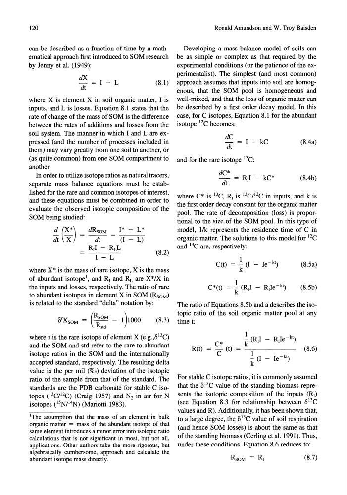
can be described as a function of time by a mathematical approach first introduced to SaM research
by Jenny et al. (1949):
dX
dt
I - L
(8.1)
where X is element X in soil organic matter, I is
inputs, and L is losses. Equation 8.1 states that the
rate of change of the mass of SaM is the difference
between the rates of additions and losses from the
soil system. The manner in which I and L are expressed (and the number of processes included in
them) may vary greatly from one soil to another, or
(as quite common) from one SaM compartment to
another.
In order to utilize isotope ratios as natural tracers,
separate mass balance equations must be established for the rare and common isotopes of interest,
and these equations must be combined in order to
evaluate the observed isotopic composition of the
saM being studied:
~ (~) = dR~~M
1*
L*
(I
L)
(8.2)
where X* is the mass of rare isotope, X is the mass
of abundant isotope 1 , and Rr and RL are X*fX in
the inputs and losses, respectively. The ratio of rare
to abundant isotopes in element X in SaM (RSOM)
is related to the standard "delta" notation by:
( RSOM
)
8IJC SOM = - - - 1 1000
Rstd
(8.3)
where r is the rare isotope of element X (e.g.,8 l3 C)
and the SaM and std refer to the rare to abundant
isotope ratios in the SaM and the internationally
accepted standard, respectively. The resulting delta
value is the per mil (%0) deviation of the isotopic
ratio of the sample from that of the standard. The
standards are the PDB carbonate for stable C isotopes (l3C/l2C) (Craig 1957) and N2 in air for N
isotopes e S N/ 14 N) (Mariotti 1983).
IThe assumption that the mass of an element in bulk
organic matter = mass of the abundant isotope of that
same element introduces a minor error into isotopic ratio
calculations that is not significant in most, but not all,
applications. Other authors take the more rigorous, but
algebraically cumbersome, approach and calculate the
abundant isotope mass directly.
Ronald Amundson and W. Troy Baisden
Developing a mass balance model of soils can
be as simple or complex as that required by the
experimental conditions (or the patience of the experimentalist). The simplest (and most common)
approach assumes that inputs into soil are homogenous, that the saM pool is homogeneous and
well-mixed, and that the loss of organic matter can
be described by a first order decay model. In this
case, for C isotopes, Equation 8.1 for the abundant
isotope 12C becomes:
dC
dt
I - kC
and for the rare isotope l3C:
dC*
-
= RrI - kC*
dt
(8.4a)
(8.4b)
where C* is l3C, Rr is l3C/ l2 C in inputs, and k is
the first order decay constant for the organic matter
pool. The rate of decomposition (loss) is proportional to the size of the SaM pool. In this type of
model, 11k represents the residence time of C in
organic matter. The solutions to this model for l2C
and l3C are, respectively:
1
C(t) = - (I - Ie- kt )
k
1
C *(t)
(R I - RrIe- kt )
= k r
(8.5a)
(S.Sb)
The ratio of Equations 8.Sb and a describes the isotopic ratio of the soil organic matter pool at any
time t:
1
RrIe- kt )
C*
k (R,I
R(t)
-(t)
1
(8.6)
C
- Ie- kt )
- (I
k
For stable C isotope ratios, it is commonly assumed
that the 8l3C value of the standing biomass represents the isotopic composition of the inputs (R,)
(see Equation 8.3 for relationship between 8 l3 C
values and R). Additionally, it has been shown that,
to a large degree, the 8l3C value of soil respiration
(and hence SaM losses) is about the same as that
of the standing biomass (Ceding et al. 1991). Thus,
under these conditions, Equation 8.6 reduces to:
(8.7)
can be described as a function of time by a mathematical approach first introduced to SaM research
by Jenny et al. (1949):
dX
dt
I - L
(8.1)
where X is element X in soil organic matter, I is
inputs, and L is losses. Equation 8.1 states that the
rate of change of the mass of SaM is the difference
between the rates of additions and losses from the
soil system. The manner in which I and L are expressed (and the number of processes included in
them) may vary greatly from one soil to another, or
(as quite common) from one SaM compartment to
another.
In order to utilize isotope ratios as natural tracers,
separate mass balance equations must be established for the rare and common isotopes of interest,
and these equations must be combined in order to
evaluate the observed isotopic composition of the
saM being studied:
~ (~) = dR~~M
1*
L*
(I
L)
(8.2)
where X* is the mass of rare isotope, X is the mass
of abundant isotope 1 , and Rr and RL are X*fX in
the inputs and losses, respectively. The ratio of rare
to abundant isotopes in element X in SaM (RSOM)
is related to the standard "delta" notation by:
( RSOM
)
8IJC SOM = - - - 1 1000
Rstd
(8.3)
where r is the rare isotope of element X (e.g.,8 l3 C)
and the SaM and std refer to the rare to abundant
isotope ratios in the SaM and the internationally
accepted standard, respectively. The resulting delta
value is the per mil (%0) deviation of the isotopic
ratio of the sample from that of the standard. The
standards are the PDB carbonate for stable C isotopes (l3C/l2C) (Craig 1957) and N2 in air for N
isotopes e S N/ 14 N) (Mariotti 1983).
IThe assumption that the mass of an element in bulk
organic matter = mass of the abundant isotope of that
same element introduces a minor error into isotopic ratio
calculations that is not significant in most, but not all,
applications. Other authors take the more rigorous, but
algebraically cumbersome, approach and calculate the
abundant isotope mass directly.
Ronald Amundson and W. Troy Baisden
Developing a mass balance model of soils can
be as simple or complex as that required by the
experimental conditions (or the patience of the experimentalist). The simplest (and most common)
approach assumes that inputs into soil are homogenous, that the saM pool is homogeneous and
well-mixed, and that the loss of organic matter can
be described by a first order decay model. In this
case, for C isotopes, Equation 8.1 for the abundant
isotope 12C becomes:
dC
dt
I - kC
and for the rare isotope l3C:
dC*
-
= RrI - kC*
dt
(8.4a)
(8.4b)
where C* is l3C, Rr is l3C/ l2 C in inputs, and k is
the first order decay constant for the organic matter
pool. The rate of decomposition (loss) is proportional to the size of the SaM pool. In this type of
model, 11k represents the residence time of C in
organic matter. The solutions to this model for l2C
and l3C are, respectively:
1
C(t) = - (I - Ie- kt )
k
1
C *(t)
(R I - RrIe- kt )
= k r
(8.5a)
(S.Sb)
The ratio of Equations 8.Sb and a describes the isotopic ratio of the soil organic matter pool at any
time t:
1
RrIe- kt )
C*
k (R,I
R(t)
-(t)
1
(8.6)
C
- Ie- kt )
- (I
k
For stable C isotope ratios, it is commonly assumed
that the 8l3C value of the standing biomass represents the isotopic composition of the inputs (R,)
(see Equation 8.3 for relationship between 8 l3 C
values and R). Additionally, it has been shown that,
to a large degree, the 8l3C value of soil respiration
(and hence SaM losses) is about the same as that
of the standing biomass (Ceding et al. 1991). Thus,
under these conditions, Equation 8.6 reduces to:
(8.7)