

370
R. Crema et aI.
sampling point. Sediments were processed
through a sieve with mesh size of 0.5 mm. The
retained material was preserved in 4% neutral
formalin in seawater. The animals were extracted
from the residual sediment and the polychaete
and mollusc fraction, which comprises over 90%
of the total macrofauna, was identified to species.
A matrix was composed comprising the number
(pooled over three replicates) of individuals of
each species at each sampling occasion and site.
A variety of structural and diversity indices were
calculated, but only the Shannon-Wiener index
will be discussed.
Three basic multivariate techniques were
used: a Factorial Analysis of Correspondences
(FAC) (Benzecr} 1982) and a Multidimensional
Scaling (MDS) (Shepard 1962) as ordination
techniques and a cluster analysis. based on the
Bray-Curtis similarity coefficient, as a classification technique (Field et al. 1982).
In addition, in both the investigated periods.
the Shannon diversity was plotted against the
sample dimension. To do this, the two sample
sets were fust sorted in order of increasing diversity, the first two ordered samples pooled and the
diversity recalculated on the pooled data. This
procedure was repeated until all the samples
were pooled together.
Results
A total of 108 polychaete and mollusc species,
reported in Table 1. were found on the two sampling occasions. Of these, 48 were common to
both periods. whereas the remaining 60 were
exclusive to the first or the second period, evidencing a great qualitative difference between
the communities of the two periods. The list and
the densities of the 10 species, common to both
periods, that exhibited the greatest variation in
abundance between the periods, are reported in
Table 2.
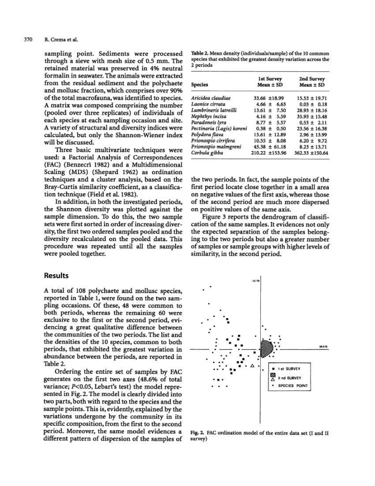
Ordering the entire set of samples by FAC
generates on the fust two axes (48.6% of total
variance; P<0.05, Lebart's test) the model represented in Fig. 2. The model is clearly divided into
two parts, both with regard to the species and the
sample points. This is, evidently, explained by the
variations undergone by the community in its
specific composition, from the first to the second
period. Moreover, the same model evidences a
different pattern of dispersion of the samples of
Table 2. Mean density (individuals/sample) of the 10 common
species that exhibited the greatest density variation across the
2 periods
Species
Aricidea claudiae
Laonice cirrata
Lumbrineris latreiUi
Nephthys incisa
Paradoneis lyra
Pectinaria (Lagis) koreni
Polydora flava
Prionospio cirrifera
Prirmospio malmgreni
Corbula gibba
1st Survey
Mean±SD
33.66 ±18.99
4.66 ± 6.63
13.61 ± 7.50
4.16 ± 5.59
8.77 ± 5.57
0.38 ± 0.50
15.61 ± 12.89
10.55 ± 8.08
45.38 ± 61.18
210.22 ±153.96
2nd Survey
Mean±SD
15.53 ± 19.71
0.03 ± 0.18
28.93 ± 18.16
35.93 ± 15.48
0.53 ± 2.11
23.56 ± 16.38
2.96 ± 13.99
6.20 ± 9.72
8.23 ± 13.71
362.33 ± 150.64
the two periods. In fact, the sample points of the
first period locate close together in a small area
on negative values of the fust axis, whereas those
of the second period are much more dispersed
on positive values of the same axis.
Figure 3 reports the dendrogram of classification of the same samples. It evidences not only
the expected separation of the samples belonging to the two periods but also a greater number
of samples or sample groups with higher levels of
similarity, in the second period.
.
.
•
•
• •
• •
• • •
.-.. ..
•
•
• III.
••
•
•
III
• •
~
.. . .. •
...
III •
38.5%
. - - - - - - -
• 1st SURVEY
,
2 nd SURVEY
• SPECIES POINT
Fig. 2. FAC ordination model of the entire data set (I and II
survey)
R. Crema et aI.
sampling point. Sediments were processed
through a sieve with mesh size of 0.5 mm. The
retained material was preserved in 4% neutral
formalin in seawater. The animals were extracted
from the residual sediment and the polychaete
and mollusc fraction, which comprises over 90%
of the total macrofauna, was identified to species.
A matrix was composed comprising the number
(pooled over three replicates) of individuals of
each species at each sampling occasion and site.
A variety of structural and diversity indices were
calculated, but only the Shannon-Wiener index
will be discussed.
Three basic multivariate techniques were
used: a Factorial Analysis of Correspondences
(FAC) (Benzecr} 1982) and a Multidimensional
Scaling (MDS) (Shepard 1962) as ordination
techniques and a cluster analysis. based on the
Bray-Curtis similarity coefficient, as a classification technique (Field et al. 1982).
In addition, in both the investigated periods.
the Shannon diversity was plotted against the
sample dimension. To do this, the two sample
sets were fust sorted in order of increasing diversity, the first two ordered samples pooled and the
diversity recalculated on the pooled data. This
procedure was repeated until all the samples
were pooled together.
Results
A total of 108 polychaete and mollusc species,
reported in Table 1. were found on the two sampling occasions. Of these, 48 were common to
both periods. whereas the remaining 60 were
exclusive to the first or the second period, evidencing a great qualitative difference between
the communities of the two periods. The list and
the densities of the 10 species, common to both
periods, that exhibited the greatest variation in
abundance between the periods, are reported in
Table 2.
Ordering the entire set of samples by FAC
generates on the fust two axes (48.6% of total
variance; P<0.05, Lebart's test) the model represented in Fig. 2. The model is clearly divided into
two parts, both with regard to the species and the
sample points. This is, evidently, explained by the
variations undergone by the community in its
specific composition, from the first to the second
period. Moreover, the same model evidences a
different pattern of dispersion of the samples of
Table 2. Mean density (individuals/sample) of the 10 common
species that exhibited the greatest density variation across the
2 periods
Species
Aricidea claudiae
Laonice cirrata
Lumbrineris latreiUi
Nephthys incisa
Paradoneis lyra
Pectinaria (Lagis) koreni
Polydora flava
Prionospio cirrifera
Prirmospio malmgreni
Corbula gibba
1st Survey
Mean±SD
33.66 ±18.99
4.66 ± 6.63
13.61 ± 7.50
4.16 ± 5.59
8.77 ± 5.57
0.38 ± 0.50
15.61 ± 12.89
10.55 ± 8.08
45.38 ± 61.18
210.22 ±153.96
2nd Survey
Mean±SD
15.53 ± 19.71
0.03 ± 0.18
28.93 ± 18.16
35.93 ± 15.48
0.53 ± 2.11
23.56 ± 16.38
2.96 ± 13.99
6.20 ± 9.72
8.23 ± 13.71
362.33 ± 150.64
the two periods. In fact, the sample points of the
first period locate close together in a small area
on negative values of the fust axis, whereas those
of the second period are much more dispersed
on positive values of the same axis.
Figure 3 reports the dendrogram of classification of the same samples. It evidences not only
the expected separation of the samples belonging to the two periods but also a greater number
of samples or sample groups with higher levels of
similarity, in the second period.
.
.
•
•
• •
• •
• • •
.-.. ..
•
•
• III.
••
•
•
III
• •
~
.. . .. •
...
III •
38.5%
. - - - - - - -
• 1st SURVEY
,
2 nd SURVEY
• SPECIES POINT
Fig. 2. FAC ordination model of the entire data set (I and II
survey)