

344
S. Schiaparelli et a1.
o
10
20
~
30
a:
I
:5
40
~
en
en
50
Ia:
::J
60
Q
I
>«
70
a:
OJ
80
90
100
6
4
2
5
3
1
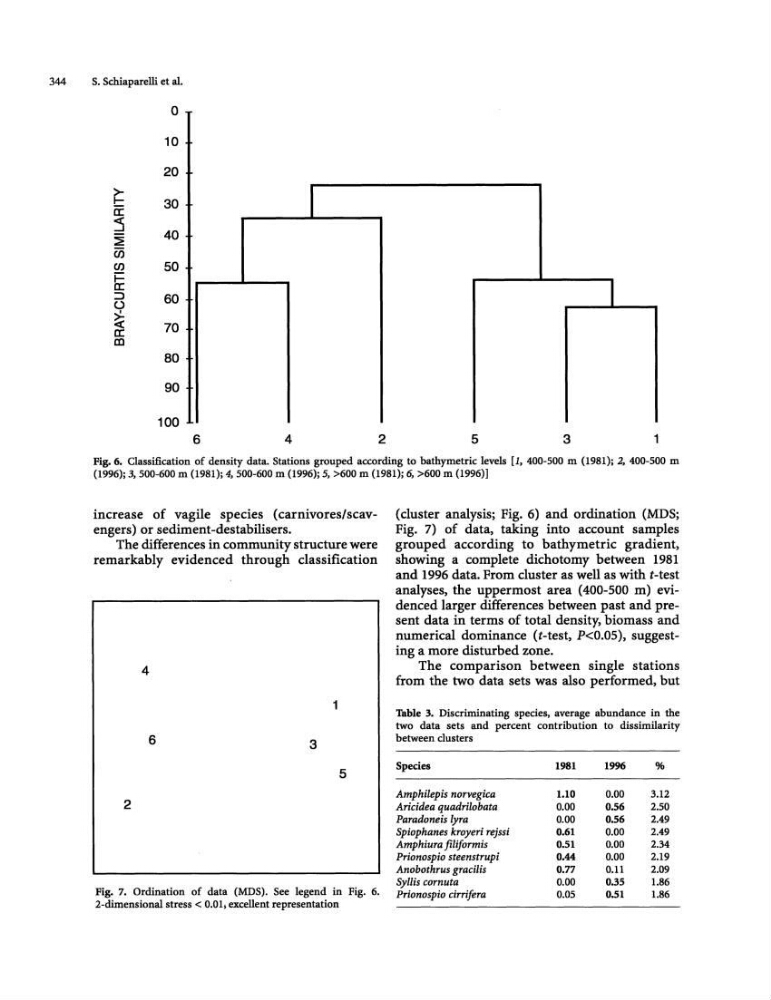
Fig.6. Classification of density data. Stations grouped according to bathymetric levels [1, 400-500 m (1981); 2, 400-500 m
(1996); 3,500-600 m (1981); 4,500-600 m (1996); 5. >600 m (1981); 6, >600 m (1996)]
increase of vagile species (carnivores/scavengers) or sediment-destabilisers.
The differences in community structure were
remarkably evidenced through classification
4
1
6
3
5
2
Fig. 7. Ordination of data (MDS). See legend in Fig. 6.
2-dimensional stress < 0.01, excellent representation
(cluster analysis; Fig. 6) and ordination (MDS;
Fig. 7) of data, taking into account samples
grouped according to bathymetric gradient,
showing a complete dichotomy between 1981
and 1996 data. From cluster as well as with t-test
analyses, the uppermost area (400-500 m) evidenced larger differences between past and present data in terms of total density, biomass and
numerical dominance (t-test, P<0.05), suggesting a more disturbed zone.
The comparison between single stations
from the two data sets was also performed. but
Table 3. Discriminating species, average abundance in the
two data sets and percent contribution to dissimilarity
between clusters
Species
1981
1996
%
Amphilepis norvegica
1.10
0.00
3.12
Aricidea quadrilobata
0.00
0.56
2.50
Paradoneis lyra
0.00
0.56
2.49
Spiophanes kroyeri rejssi
0.61
0.00
2.49
Amphiura filiformis
0.51
0.00
2.34
Prionospio steenstrupi
0.44
0.00
2.19
Anobothrus gracilis
0.77
0.11
2.09
Syllis corn uta
0.00
0.35
1.86
Prionospio cirrifera
0.05
0.51
1.86
S. Schiaparelli et a1.
o
10
20
~
30
a:
I
:5
40
~
en
en
50
Ia:
::J
60
Q
I
>«
70
a:
OJ
80
90
100
6
4
2
5
3
1
Fig.6. Classification of density data. Stations grouped according to bathymetric levels [1, 400-500 m (1981); 2, 400-500 m
(1996); 3,500-600 m (1981); 4,500-600 m (1996); 5. >600 m (1981); 6, >600 m (1996)]
increase of vagile species (carnivores/scavengers) or sediment-destabilisers.
The differences in community structure were
remarkably evidenced through classification
4
1
6
3
5
2
Fig. 7. Ordination of data (MDS). See legend in Fig. 6.
2-dimensional stress < 0.01, excellent representation
(cluster analysis; Fig. 6) and ordination (MDS;
Fig. 7) of data, taking into account samples
grouped according to bathymetric gradient,
showing a complete dichotomy between 1981
and 1996 data. From cluster as well as with t-test
analyses, the uppermost area (400-500 m) evidenced larger differences between past and present data in terms of total density, biomass and
numerical dominance (t-test, P<0.05), suggesting a more disturbed zone.
The comparison between single stations
from the two data sets was also performed. but
Table 3. Discriminating species, average abundance in the
two data sets and percent contribution to dissimilarity
between clusters
Species
1981
1996
%
Amphilepis norvegica
1.10
0.00
3.12
Aricidea quadrilobata
0.00
0.56
2.50
Paradoneis lyra
0.00
0.56
2.49
Spiophanes kroyeri rejssi
0.61
0.00
2.49
Amphiura filiformis
0.51
0.00
2.34
Prionospio steenstrupi
0.44
0.00
2.19
Anobothrus gracilis
0.77
0.11
2.09
Syllis corn uta
0.00
0.35
1.86
Prionospio cirrifera
0.05
0.51
1.86