

4.3 Statistical Methods
67
60
N
608 x
~
6x~
0
8"
fr7'$ 07
08
0
7+7
"3 +3
63"4L>4
3x 4°4x 40 +4
30
-1
-1
0
2
DIM(1)
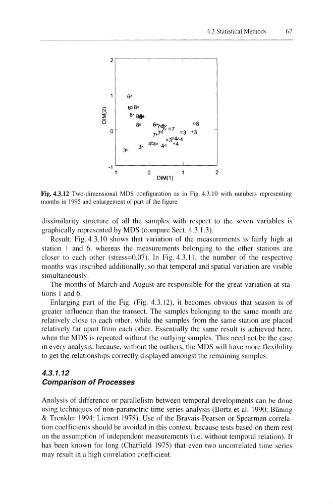
Fig. 4.3.12 Two-dimensional MDS configuration as in Fig. 4.3.10 with numbers representing
months in 1995 and enlargement of part of the figure
dissimilarity structure of all the samples with respect to the seven variables is
graphically represented by MDS (compare Sect. 4.3.1.3).
Result: Fig. 4.3.10 shows that variation of the measurements is fairly high at
station I and 6, whereas the measurements belonging to the other stations are
closer to each other (stress=0.07). In Fig. 4.3.11, the number of the respective
months was inscribed additionally, so that temporal and spatial variation are visible
simultaneously.
The months of March and August are responsible for the great variation at stations I and 6.
Enlarging part of the Fig. (Fig. 4.3.12), it becomes obvious that season is of
greater influence than the transect. The samples belonging to the same month are
relatively close to each other, while the samples from the same station are placed
relatively far apart from each other. Essentially the same result is achieved here,
when the MDS is repeated without the outlying samples. This need not be the case
in every analysis, because, without the outliers, the MDS will have more flexibility
to get the relationships correctly displayed amongst the remaining samples.
4.3.1.12
Comparison of Processes
Analysis of difference or parallelism between temporal developments can be done
using techniques of non-parametric time series analysis (Bortz et al. 1990; Bi.ining
& Trenkler 1994; Lienert 1978). Use of the Bravais-Pearson or Spearman correlation coefficients should be avoided in this context, because tests based on them rest
on the assumption of independent measurements (i.e. without temporal relation). It
has been known for long (Chatfield 1975) that even two uncorrelated time series
may result in a high correlation coefficient.
67
60
N
608 x
~
6x~
0
8"
fr7'$ 07
08
0
7+7
"3 +3
63"4L>4
3x 4°4x 40 +4
30
-1
-1
0
2
DIM(1)
Fig. 4.3.12 Two-dimensional MDS configuration as in Fig. 4.3.10 with numbers representing
months in 1995 and enlargement of part of the figure
dissimilarity structure of all the samples with respect to the seven variables is
graphically represented by MDS (compare Sect. 4.3.1.3).
Result: Fig. 4.3.10 shows that variation of the measurements is fairly high at
station I and 6, whereas the measurements belonging to the other stations are
closer to each other (stress=0.07). In Fig. 4.3.11, the number of the respective
months was inscribed additionally, so that temporal and spatial variation are visible
simultaneously.
The months of March and August are responsible for the great variation at stations I and 6.
Enlarging part of the Fig. (Fig. 4.3.12), it becomes obvious that season is of
greater influence than the transect. The samples belonging to the same month are
relatively close to each other, while the samples from the same station are placed
relatively far apart from each other. Essentially the same result is achieved here,
when the MDS is repeated without the outlying samples. This need not be the case
in every analysis, because, without the outliers, the MDS will have more flexibility
to get the relationships correctly displayed amongst the remaining samples.
4.3.1.12
Comparison of Processes
Analysis of difference or parallelism between temporal developments can be done
using techniques of non-parametric time series analysis (Bortz et al. 1990; Bi.ining
& Trenkler 1994; Lienert 1978). Use of the Bravais-Pearson or Spearman correlation coefficients should be avoided in this context, because tests based on them rest
on the assumption of independent measurements (i.e. without temporal relation). It
has been known for long (Chatfield 1975) that even two uncorrelated time series
may result in a high correlation coefficient.