

60
4 Statistical Models and Techniques
ard error is at least a 75 % confidence interval for the mean (by the Tschebyscheff
inequality). If the intervals belonging to two samples intersect, a respective statistical test will not reject the null hypothesis of equality of the two location parameters.
In the multivariate case, the variables should be represented simultaneously in a
figure, i.e. from the representation one should be able to see which values of several variables were assumed at the same sample. As in the univariate case, a variance interval of the distribution and a confidence interval for the common location
parameter can be computed. Both require knowledge about the two-dimensional
distribution. In common statistical software packages, a multivariate normal distribution is generally assumed. The confidence region is a (multidimensional) ellipse,
whose length and width are determined by the standard deviation of the variables
and its orientation is determined by the covariance of the two variables. In the
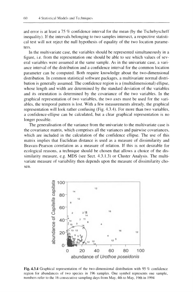
graphical representation of two variables, the two axes must be used for the variables, the temporal pattern is lost. With a few measurements already, the graphical
representation will look rather confusing (Fig. 4.3.4). For more than two variables,
a confidence-ellipse can be calculated, but a clear graphical representation is no
longer possible.
The generalisation of the variance from the univariate to the multivariate case is
the covariance matrix, which comprises all the variances and pairwise covariances,
which are included in the calculation of the confidence ellipse. The use of this
matrix implies that Euclidean distance is used as a measure of dissimilarity and
Bravais-Pearson correlation as a measure of relation. If this is not desirable for
ecological reasons, a technique should be chosen that allows a choice of the dissimilarity measure, e.g. MDS (see Sect. 4.3.1.3) or Cluster Analysis. The multivariate measure of variability then depends upon the measure of dissimilarity chosen.
~1
~
~
"
Co)
80
12
Jg
12
~ 60
0..
(I]
<.:>
16
..... 0
Q)
<.J
c:
<0
"0
16
12
c:
::J
.0
12 5
<0
0
20
40
60
80
100
abundance of Urothoe poseidonis
Fig. 4.3.4 Graphical representation of the two-dimensional distribution with 95 % confidence
region for abundances of two species in 196 samples. One symbol represents one sample,
numbers refer to the 16 consecutive sampling days from May, 4th to May, 19th in 1994
4 Statistical Models and Techniques
ard error is at least a 75 % confidence interval for the mean (by the Tschebyscheff
inequality). If the intervals belonging to two samples intersect, a respective statistical test will not reject the null hypothesis of equality of the two location parameters.
In the multivariate case, the variables should be represented simultaneously in a
figure, i.e. from the representation one should be able to see which values of several variables were assumed at the same sample. As in the univariate case, a variance interval of the distribution and a confidence interval for the common location
parameter can be computed. Both require knowledge about the two-dimensional
distribution. In common statistical software packages, a multivariate normal distribution is generally assumed. The confidence region is a (multidimensional) ellipse,
whose length and width are determined by the standard deviation of the variables
and its orientation is determined by the covariance of the two variables. In the
graphical representation of two variables, the two axes must be used for the variables, the temporal pattern is lost. With a few measurements already, the graphical
representation will look rather confusing (Fig. 4.3.4). For more than two variables,
a confidence-ellipse can be calculated, but a clear graphical representation is no
longer possible.
The generalisation of the variance from the univariate to the multivariate case is
the covariance matrix, which comprises all the variances and pairwise covariances,
which are included in the calculation of the confidence ellipse. The use of this
matrix implies that Euclidean distance is used as a measure of dissimilarity and
Bravais-Pearson correlation as a measure of relation. If this is not desirable for
ecological reasons, a technique should be chosen that allows a choice of the dissimilarity measure, e.g. MDS (see Sect. 4.3.1.3) or Cluster Analysis. The multivariate measure of variability then depends upon the measure of dissimilarity chosen.
~1
~
~
"
Co)
80
12
Jg
12
~ 60
0..
(I]
<.:>
16
..... 0
Q)
<.J
c:
<0
"0
16
12
c:
::J
.0
12 5
<0
0
20
40
60
80
100
abundance of Urothoe poseidonis
Fig. 4.3.4 Graphical representation of the two-dimensional distribution with 95 % confidence
region for abundances of two species in 196 samples. One symbol represents one sample,
numbers refer to the 16 consecutive sampling days from May, 4th to May, 19th in 1994