

ISO
5 Spallal and Temporal DIstnhutJ()n Patterns
recruitment and, if necessary, density dependence, mortality is taken into account.
Each individual (including those newly established) has the probability Pmort
(= 0.5) of dying.
In the following, the results of simulating a one-metre-long transect (i.e., a hundred grid cells) are presented. Simulations start with five randomly distributed
tubes. Fig. 5.4.2 shows three ways of visualizing the distribution of the tubes. In
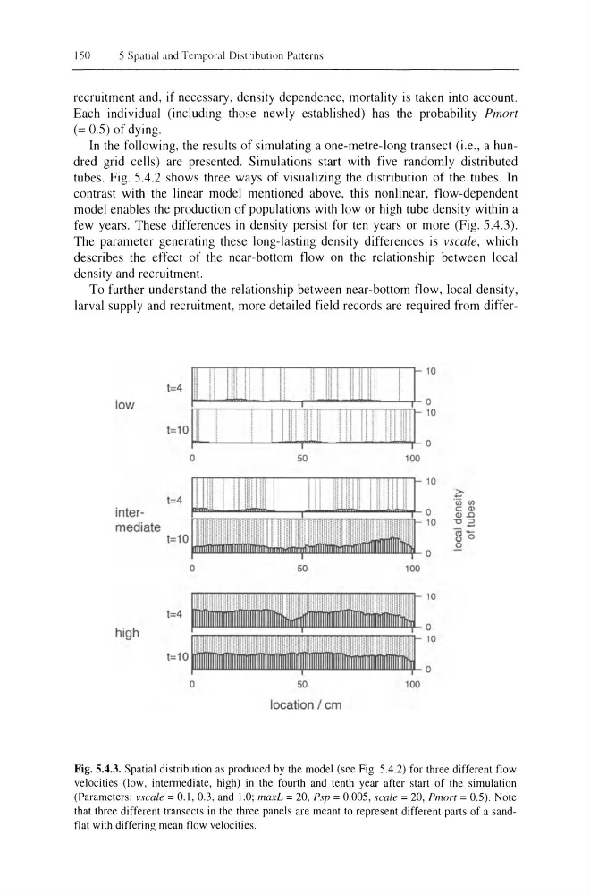
contrast with the linear model mentioned above, this nonlinear, flow-dependent
model enables the production of populations with low or high tube density within a
few years. These differences in density persist for ten years or more (Fig. 5.4.3).
The parameter generating these long-lasting density differences is vscale, which
describes the effect of the near-bottom flow on the relationship between local
density and recruitment.
To further understand the relationship between near-bottom flow, local density,
larval supply and recruitment, more detailed field records are required from differ10
1=4
low
0
10
1=10
0
0
50
100
10
1=4
.2='
"(j) t.n
inter0
C Q)
Q),C
mediate
10
"02
(ij1",10
0 0
.2
0
0
50
100
10
1",4
high
0
10
l",tO
0
0
50
100
location / em
Fig. 5.4.3. Spatial distrihution as produced hy the model (see Fig. 5.4.2) for three different flow
velocities (low, intermediate, high) in the fourth and tenth year after start of the simulation
(Parameters: vscale = 0.1, 0.3, and 1.0; maxL = 20, Psp = 0.005, scale = 20, Pmort = 0.5). Note
that three different transects in the three panels are meant to represent different parts of a sandflat with differing mean flow velocities.
5 Spallal and Temporal DIstnhutJ()n Patterns
recruitment and, if necessary, density dependence, mortality is taken into account.
Each individual (including those newly established) has the probability Pmort
(= 0.5) of dying.
In the following, the results of simulating a one-metre-long transect (i.e., a hundred grid cells) are presented. Simulations start with five randomly distributed
tubes. Fig. 5.4.2 shows three ways of visualizing the distribution of the tubes. In
contrast with the linear model mentioned above, this nonlinear, flow-dependent
model enables the production of populations with low or high tube density within a
few years. These differences in density persist for ten years or more (Fig. 5.4.3).
The parameter generating these long-lasting density differences is vscale, which
describes the effect of the near-bottom flow on the relationship between local
density and recruitment.
To further understand the relationship between near-bottom flow, local density,
larval supply and recruitment, more detailed field records are required from differ10
1=4
low
0
10
1=10
0
0
50
100
10
1=4
.2='
"(j) t.n
inter0
C Q)
Q),C
mediate
10
"02
(ij1",10
0 0
.2
0
0
50
100
10
1",4
high
0
10
l",tO
0
0
50
100
location / em
Fig. 5.4.3. Spatial distrihution as produced hy the model (see Fig. 5.4.2) for three different flow
velocities (low, intermediate, high) in the fourth and tenth year after start of the simulation
(Parameters: vscale = 0.1, 0.3, and 1.0; maxL = 20, Psp = 0.005, scale = 20, Pmort = 0.5). Note
that three different transects in the three panels are meant to represent different parts of a sandflat with differing mean flow velocities.