

315
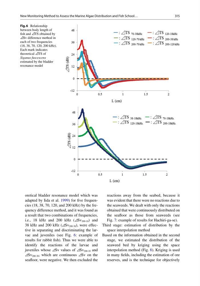
oretical bladder resonance model which was
adapted by Iida et al. 1999 ) for fi ve frequencies (18, 38, 70, 120, and 200 kHz) by the frequency difference method, and it was found as
a result that two combinations of frequencies,
i.e., 18 kHz and 200 kHz ( ⊿ Sv 200-18 ) and
38 kHz and 200 kHz (⊿Sv 200-38 ), were effective in separating and discriminating the larvae and juveniles (see Fig. 6 : example of
results for rabbit fi sh). Thus we were able to
identify the reactions of the larvae and
juveniles whose ⊿Sv values of ⊿Sv 200-18 and
⊿ Sv 200-38 , which are continuous ⊿ Sv on the
seafl oor, were negative. We then excluded the
reactions away from the seabed, because it
was evident that there were no reactions due to
the seaweeds. We dealt with only the reactions
obtained that were continuously distributed on
the seafl oor as those from seaweeds (see
Fig. 7 : example of results for Hachiri-ga-se).
Third stage: estimation of distribution by the
space interpolation method
Based on the information obtained in the second
stage, we estimated the distribution of the
seaweed bed by kriging using the space
interpolation method (Fig. 8 ). Kriging is used
in many fi elds, including the estimation of ore
reserves, and is the technique for objectively
Fig. 6 Relationship
between body length of
fi sh and ⊿ TS obtained by
⊿ Sv difference method in
each of two frequencies
(18, 38, 70, 120, 200 kHz).
Each mark indicates
theoretical ⊿ TS of
Siganus fuscescens
estimated by the bladder
resonance model
New Monitoring Method to Assess the Marine Algae Distribution and Fish School…
oretical bladder resonance model which was
adapted by Iida et al. 1999 ) for fi ve frequencies (18, 38, 70, 120, and 200 kHz) by the frequency difference method, and it was found as
a result that two combinations of frequencies,
i.e., 18 kHz and 200 kHz ( ⊿ Sv 200-18 ) and
38 kHz and 200 kHz (⊿Sv 200-38 ), were effective in separating and discriminating the larvae and juveniles (see Fig. 6 : example of
results for rabbit fi sh). Thus we were able to
identify the reactions of the larvae and
juveniles whose ⊿Sv values of ⊿Sv 200-18 and
⊿ Sv 200-38 , which are continuous ⊿ Sv on the
seafl oor, were negative. We then excluded the
reactions away from the seabed, because it
was evident that there were no reactions due to
the seaweeds. We dealt with only the reactions
obtained that were continuously distributed on
the seafl oor as those from seaweeds (see
Fig. 7 : example of results for Hachiri-ga-se).
Third stage: estimation of distribution by the
space interpolation method
Based on the information obtained in the second
stage, we estimated the distribution of the
seaweed bed by kriging using the space
interpolation method (Fig. 8 ). Kriging is used
in many fi elds, including the estimation of ore
reserves, and is the technique for objectively
Fig. 6 Relationship
between body length of
fi sh and ⊿ TS obtained by
⊿ Sv difference method in
each of two frequencies
(18, 38, 70, 120, 200 kHz).
Each mark indicates
theoretical ⊿ TS of
Siganus fuscescens
estimated by the bladder
resonance model
New Monitoring Method to Assess the Marine Algae Distribution and Fish School…