

192
3.3
Fishing and Fleet Behavior
The strategy of a fleet is the pattern of effort allocation over métiers along the year. Initially, the
model is set by computing the average effort per
fleet, gear, and month based on logbooks for the
period 2008–2010 and then further allocated spatially (either by ISIS-polygons or ICES- rectangles).
The strategy is supposed to change in response to
species availability, economic, and management
constraints. Therefore, a gravity model is used to
predict the changes in effort allocation over métiers
within a strategy. Following Marchal et al. (2011),
the proportion P of effort allocated to a métier is a
linear combination of proxies for opportunism and
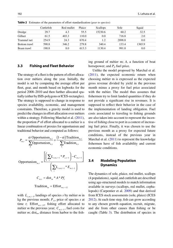
traditional behavior and computed as follows:
P m t
m t
k
k t
m t
k
,
,
,
,
=
+
−
( )
∑
∑
a
a
Opportunism
Opportunism
Tradition
Tr
1
a adition k t
,
Opportunism m t
s
s m t
st
m t
s
s m
L
P
C
L
,
, ,
,
,
, ,
*
=
−
∑
∑
−
−
−
1
1
1
t t
m t
E
−
−
1
1
* ,
C
A Pf
m t
m
t
,
* *
= dist
Tradition
Effort
m
m t
=
−
, 12
with L s m t
, , −1 , landings of species s by métier m in
kg the previous month; P s,t , price of species s at
time t; Effort m t
, −12 , fishing effort allocated to
métier m the previous year; C m t
, −1 , fuel costs for
métier m; dist m , distance from harbor to the fishing ground of métier m; A, a function of boat
horsepower; and P ft fuel price.
Unlike the model proposed by Marchal et al.
(2011), the expected economic return when
choosing métier m is expressed as the expected
gross revenue divided by yield in the previous
month minus a proxy for fuel price associated
with the métier. The model thus assumes that
fishermen try to limit landed quantities if they do
not provide a significant rise in revenues. It is
supposed to reflect their behavior in the case of
the implementation of landing obligation. Fuel
costs associated to traveling to fishing grounds
are also taken into account to represent the incentive of fishing close to port in a context of increasing fuel price. Finally, it was chosen to use the
previous month as a proxy for expected future
conditions, instead of the previous year in
Marchal et al. (2011) to represent the knowledge
fishermen have of fish availability and current
economic conditions.
3.4
Modeling Population
Dynamics
The dynamics of sole, plaice, red mullet, scallops
(4 populations), squid, and cuttlefish are described
using age-structured models to match information
available in surveys (scallops, red mullet, cephalopods) (Carpentier et al. 2009) and that derived
from ICES stock assessments (sole, plaice) (ICES
2012). At each time step, fish can grow according
to any chosen growth equation, recruit, migrate,
and die from other causes than fishing or be
caught (Table 3). The distribution of species in
Table 2 Estimates of the parameters of effort standardization (gear to species)
Cuttlefish
Red mullet Plaice
Scallops
Sole
Squid
Dredge
29.7
4.3
55.5
15230.6
60.2
32.5
Gillnet
61.5
403.3
110.0
0.0
716.8
2.0
Trammel net
254.9
24.3
670.4
1.2
2898.8
0.0
Bottom trawl
590.8
346.2
279.8
340.4
133.4
1365.9
Beam trawl
190.8
8.0
613.3
1130.4
991.0
0.0
S. Lehuta et al.
3.3
Fishing and Fleet Behavior
The strategy of a fleet is the pattern of effort allocation over métiers along the year. Initially, the
model is set by computing the average effort per
fleet, gear, and month based on logbooks for the
period 2008–2010 and then further allocated spatially (either by ISIS-polygons or ICES- rectangles).
The strategy is supposed to change in response to
species availability, economic, and management
constraints. Therefore, a gravity model is used to
predict the changes in effort allocation over métiers
within a strategy. Following Marchal et al. (2011),
the proportion P of effort allocated to a métier is a
linear combination of proxies for opportunism and
traditional behavior and computed as follows:
P m t
m t
k
k t
m t
k
,
,
,
,
=
+
−
( )
∑
∑
a
a
Opportunism
Opportunism
Tradition
Tr
1
a adition k t
,
Opportunism m t
s
s m t
st
m t
s
s m
L
P
C
L
,
, ,
,
,
, ,
*
=
−
∑
∑
−
−
−
1
1
1
t t
m t
E
−
−
1
1
* ,
C
A Pf
m t
m
t
,
* *
= dist
Tradition
Effort
m
m t
=
−
, 12
with L s m t
, , −1 , landings of species s by métier m in
kg the previous month; P s,t , price of species s at
time t; Effort m t
, −12 , fishing effort allocated to
métier m the previous year; C m t
, −1 , fuel costs for
métier m; dist m , distance from harbor to the fishing ground of métier m; A, a function of boat
horsepower; and P ft fuel price.
Unlike the model proposed by Marchal et al.
(2011), the expected economic return when
choosing métier m is expressed as the expected
gross revenue divided by yield in the previous
month minus a proxy for fuel price associated
with the métier. The model thus assumes that
fishermen try to limit landed quantities if they do
not provide a significant rise in revenues. It is
supposed to reflect their behavior in the case of
the implementation of landing obligation. Fuel
costs associated to traveling to fishing grounds
are also taken into account to represent the incentive of fishing close to port in a context of increasing fuel price. Finally, it was chosen to use the
previous month as a proxy for expected future
conditions, instead of the previous year in
Marchal et al. (2011) to represent the knowledge
fishermen have of fish availability and current
economic conditions.
3.4
Modeling Population
Dynamics
The dynamics of sole, plaice, red mullet, scallops
(4 populations), squid, and cuttlefish are described
using age-structured models to match information
available in surveys (scallops, red mullet, cephalopods) (Carpentier et al. 2009) and that derived
from ICES stock assessments (sole, plaice) (ICES
2012). At each time step, fish can grow according
to any chosen growth equation, recruit, migrate,
and die from other causes than fishing or be
caught (Table 3). The distribution of species in
Table 2 Estimates of the parameters of effort standardization (gear to species)
Cuttlefish
Red mullet Plaice
Scallops
Sole
Squid
Dredge
29.7
4.3
55.5
15230.6
60.2
32.5
Gillnet
61.5
403.3
110.0
0.0
716.8
2.0
Trammel net
254.9
24.3
670.4
1.2
2898.8
0.0
Bottom trawl
590.8
346.2
279.8
340.4
133.4
1365.9
Beam trawl
190.8
8.0
613.3
1130.4
991.0
0.0
S. Lehuta et al.