

177
PUs
Z PUs
Connectivity costs
Cost BLM
B oundary Cost
∑
∑∑
+
×
+
×
∑
Ft
FPF FeaturePenalty,
(1)
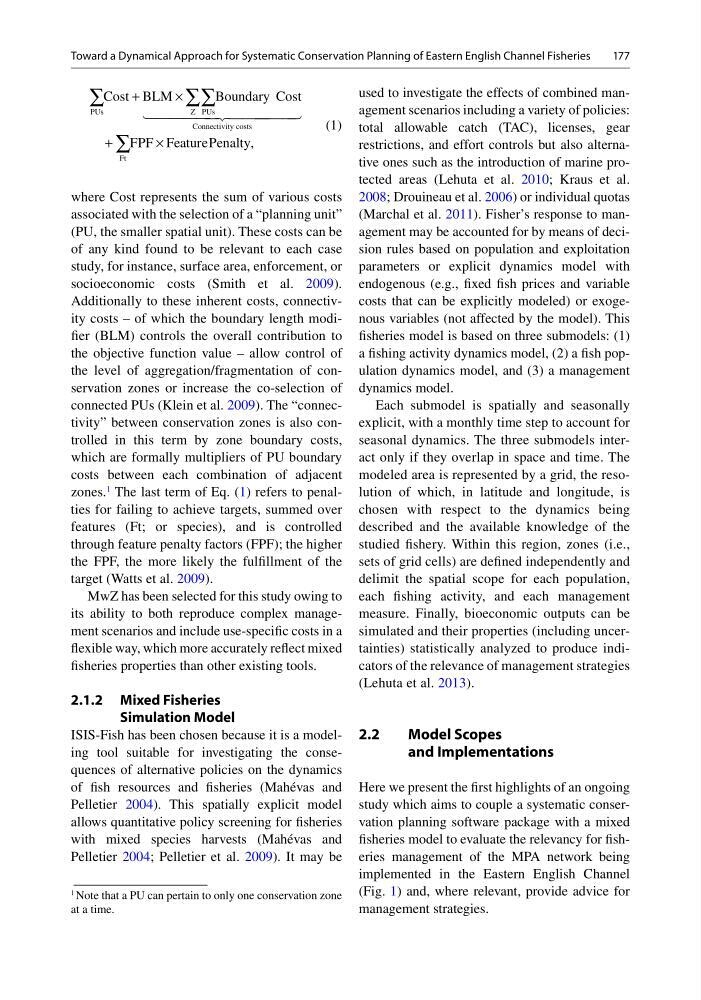
where Cost represents the sum of various costs
associated with the selection of a “planning unit”
(PU, the smaller spatial unit). These costs can be
of any kind found to be relevant to each case
study, for instance, surface area, enforcement, or
socioeconomic costs (Smith et al. 2009).
Additionally to these inherent costs, connectivity costs – of which the boundary length modifier (BLM) controls the overall contribution to
the objective function value – allow control of
the level of aggregation/fragmentation of conservation zones or increase the co-selection of
connected PUs (Klein et al. 2009). The “connectivity” between conservation zones is also controlled in this term by zone boundary costs,
which are formally multipliers of PU boundary
costs between each combination of adjacent
zones.
1
The last term of Eq. (1) refers to penalties for failing to achieve targets, summed over
features (Ft; or species), and is controlled
through feature penalty factors (FPF); the higher
the FPF, the more likely the fulfillment of the
target (Watts et al. 2009).
MwZ has been selected for this study owing to
its ability to both reproduce complex management scenarios and include use-specific costs in a
flexible way, which more accurately reflect mixed
fisheries properties than other existing tools.
2.1.2 Mixed Fisheries
Simulation Model
ISIS-Fish has been chosen because it is a modeling tool suitable for investigating the consequences of alternative policies on the dynamics
of fish resources and fisheries (Mahévas and
Pelletier 2004). This spatially explicit model
allows quantitative policy screening for fisheries
with mixed species harvests (Mahévas and
Pelletier 2004; Pelletier et al. 2009). It may be
1 Note that a PU can pertain to only one conservation zone
at a time.
used to investigate the effects of combined management scenarios including a variety of policies:
total allowable catch (TAC), licenses, gear
restrictions, and effort controls but also alternative ones such as the introduction of marine protected areas (Lehuta et al. 2010; Kraus et al.
2008; Drouineau et al. 2006) or individual quotas
(Marchal et al. 2011). Fisher’s response to management may be accounted for by means of decision rules based on population and exploitation
parameters or explicit dynamics model with
endogenous (e.g., fixed fish prices and variable
costs that can be explicitly modeled) or exogenous variables (not affected by the model). This
fisheries model is based on three submodels: (1)
a fishing activity dynamics model, (2) a fish population dynamics model, and (3) a management
dynamics model.
Each submodel is spatially and seasonally
explicit, with a monthly time step to account for
seasonal dynamics. The three submodels interact only if they overlap in space and time. The
modeled area is represented by a grid, the resolution of which, in latitude and longitude, is
chosen with respect to the dynamics being
described and the available knowledge of the
studied fishery. Within this region, zones (i.e.,
sets of grid cells) are defined independently and
delimit the spatial scope for each population,
each fishing activity, and each management
measure. Finally, bioeconomic outputs can be
simulated and their properties (including uncertainties) statistically analyzed to produce indicators of the relevance of management strategies
(Lehuta et al. 2013).
2.2
Model Scopes
and Implementations
Here we present the first highlights of an ongoing
study which aims to couple a systematic conservation planning software package with a mixed
fisheries model to evaluate the relevancy for fisheries management of the MPA network being
implemented in the Eastern English Channel
(Fig. 1) and, where relevant, provide advice for
management strategies.
Toward a Dynamical Approach for Systematic Conservation Planning of Eastern English Channel Fisheries
PUs
Z PUs
Connectivity costs
Cost BLM
B oundary Cost
∑
∑∑
+
×
+
×
∑
Ft
FPF FeaturePenalty,
(1)
where Cost represents the sum of various costs
associated with the selection of a “planning unit”
(PU, the smaller spatial unit). These costs can be
of any kind found to be relevant to each case
study, for instance, surface area, enforcement, or
socioeconomic costs (Smith et al. 2009).
Additionally to these inherent costs, connectivity costs – of which the boundary length modifier (BLM) controls the overall contribution to
the objective function value – allow control of
the level of aggregation/fragmentation of conservation zones or increase the co-selection of
connected PUs (Klein et al. 2009). The “connectivity” between conservation zones is also controlled in this term by zone boundary costs,
which are formally multipliers of PU boundary
costs between each combination of adjacent
zones.
1
The last term of Eq. (1) refers to penalties for failing to achieve targets, summed over
features (Ft; or species), and is controlled
through feature penalty factors (FPF); the higher
the FPF, the more likely the fulfillment of the
target (Watts et al. 2009).
MwZ has been selected for this study owing to
its ability to both reproduce complex management scenarios and include use-specific costs in a
flexible way, which more accurately reflect mixed
fisheries properties than other existing tools.
2.1.2 Mixed Fisheries
Simulation Model
ISIS-Fish has been chosen because it is a modeling tool suitable for investigating the consequences of alternative policies on the dynamics
of fish resources and fisheries (Mahévas and
Pelletier 2004). This spatially explicit model
allows quantitative policy screening for fisheries
with mixed species harvests (Mahévas and
Pelletier 2004; Pelletier et al. 2009). It may be
1 Note that a PU can pertain to only one conservation zone
at a time.
used to investigate the effects of combined management scenarios including a variety of policies:
total allowable catch (TAC), licenses, gear
restrictions, and effort controls but also alternative ones such as the introduction of marine protected areas (Lehuta et al. 2010; Kraus et al.
2008; Drouineau et al. 2006) or individual quotas
(Marchal et al. 2011). Fisher’s response to management may be accounted for by means of decision rules based on population and exploitation
parameters or explicit dynamics model with
endogenous (e.g., fixed fish prices and variable
costs that can be explicitly modeled) or exogenous variables (not affected by the model). This
fisheries model is based on three submodels: (1)
a fishing activity dynamics model, (2) a fish population dynamics model, and (3) a management
dynamics model.
Each submodel is spatially and seasonally
explicit, with a monthly time step to account for
seasonal dynamics. The three submodels interact only if they overlap in space and time. The
modeled area is represented by a grid, the resolution of which, in latitude and longitude, is
chosen with respect to the dynamics being
described and the available knowledge of the
studied fishery. Within this region, zones (i.e.,
sets of grid cells) are defined independently and
delimit the spatial scope for each population,
each fishing activity, and each management
measure. Finally, bioeconomic outputs can be
simulated and their properties (including uncertainties) statistically analyzed to produce indicators of the relevance of management strategies
(Lehuta et al. 2013).
2.2
Model Scopes
and Implementations
Here we present the first highlights of an ongoing
study which aims to couple a systematic conservation planning software package with a mixed
fisheries model to evaluate the relevancy for fisheries management of the MPA network being
implemented in the Eastern English Channel
(Fig. 1) and, where relevant, provide advice for
management strategies.
Toward a Dynamical Approach for Systematic Conservation Planning of Eastern English Channel Fisheries