

Imagine a ball lying at the top of this surface, such as at point A. The ball may lie
still, and very small nudges away from its equilibrium point A lead to a new
equilibrium. After a series of such small perturbations, however, the ball will roll
off the top part of the surface, and a priori, it is difficult for us to determine exactly
where it will end up. All we know for certain is that the new equilibrium position is
somewhere at the bottom of the surface, say point B.
Small nudges to the ball in B will again move it slightly away from B. And if we
kick it hard enough, we can propel the ball through the fold, or “cusp,” to the upper
part of the surface again. Where exactly will it end up? To give a precise answer
requires exact knowledge of the shape of the surface, the properties of the ball, and
the magnitude and direction of the force exerted on the ball. In more complicated,
real-life systems, not all the variables to describe the system and the forces incident
upon them are well enough known. As a result, we may only know stability
domains rather than specific locations.
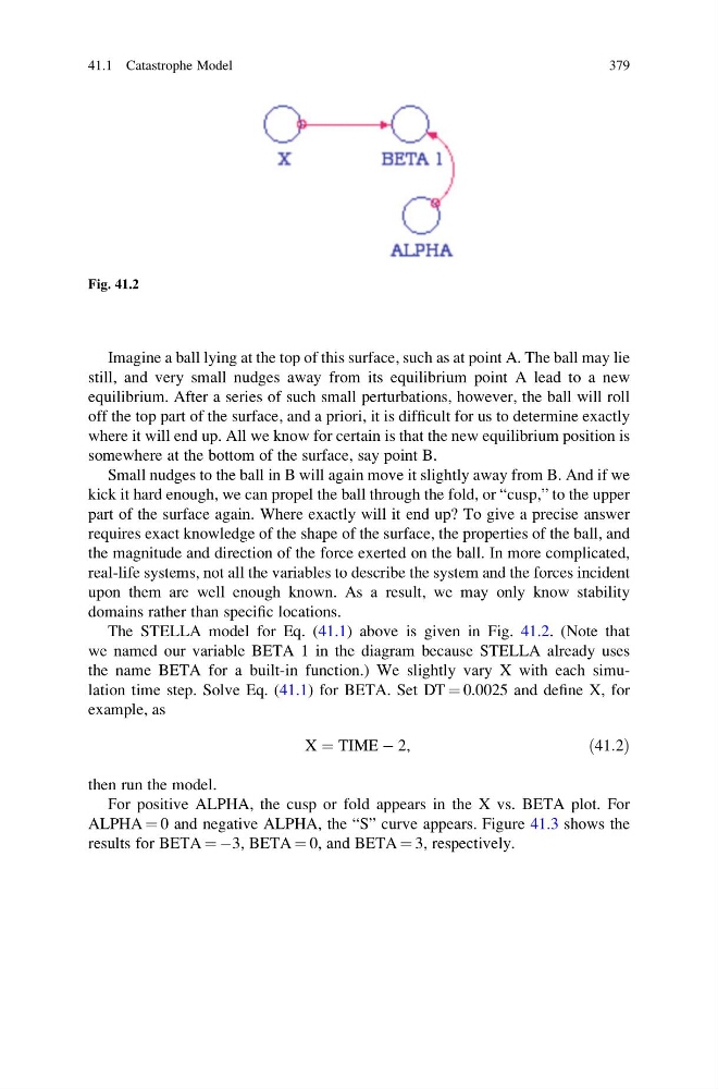
The STELLA model for Eq. (41.1) above is given in Fig. 41.2. (Note that
we named our variable BETA 1 in the diagram because STELLA already uses
the name BETA for a built-in function.) We slightly vary X with each simulation time step. Solve Eq. (41.1) for BETA. Set DT ¼ 0.0025 and define X, for
example, as
X ¼ TIME À 2,
ð41:2Þ
then run the model.
For positive ALPHA, the cusp or fold appears in the X vs. BETA plot. For
ALPHA ¼ 0 and negative ALPHA, the “S” curve appears. Figure 41.3 shows the
results for BETA ¼ À3, BETA ¼ 0, and BETA ¼ 3, respectively.
Fig. 41.2
41.1 Catastrophe Model
379
still, and very small nudges away from its equilibrium point A lead to a new
equilibrium. After a series of such small perturbations, however, the ball will roll
off the top part of the surface, and a priori, it is difficult for us to determine exactly
where it will end up. All we know for certain is that the new equilibrium position is
somewhere at the bottom of the surface, say point B.
Small nudges to the ball in B will again move it slightly away from B. And if we
kick it hard enough, we can propel the ball through the fold, or “cusp,” to the upper
part of the surface again. Where exactly will it end up? To give a precise answer
requires exact knowledge of the shape of the surface, the properties of the ball, and
the magnitude and direction of the force exerted on the ball. In more complicated,
real-life systems, not all the variables to describe the system and the forces incident
upon them are well enough known. As a result, we may only know stability
domains rather than specific locations.
The STELLA model for Eq. (41.1) above is given in Fig. 41.2. (Note that
we named our variable BETA 1 in the diagram because STELLA already uses
the name BETA for a built-in function.) We slightly vary X with each simulation time step. Solve Eq. (41.1) for BETA. Set DT ¼ 0.0025 and define X, for
example, as
X ¼ TIME À 2,
ð41:2Þ
then run the model.
For positive ALPHA, the cusp or fold appears in the X vs. BETA plot. For
ALPHA ¼ 0 and negative ALPHA, the “S” curve appears. Figure 41.3 shows the
results for BETA ¼ À3, BETA ¼ 0, and BETA ¼ 3, respectively.
Fig. 41.2
41.1 Catastrophe Model
379