

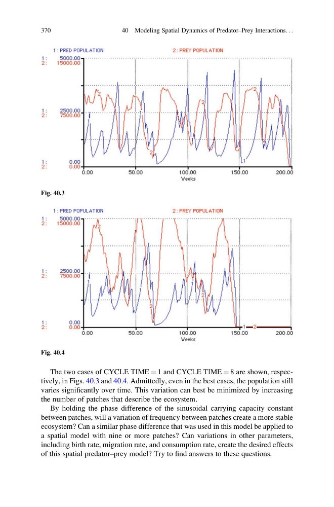
The two cases of CYCLE TIME ¼ 1 and CYCLE TIME ¼ 8 are shown, respectively, in Figs. 40.3 and 40.4. Admittedly, even in the best cases, the population still
varies significantly over time. This variation can best be minimized by increasing
the number of patches that describe the ecosystem.
By holding the phase difference of the sinusoidal carrying capacity constant
between patches, will a variation of frequency between patches create a more stable
ecosystem? Can a similar phase difference that was used in this model be applied to
a spatial model with nine or more patches? Can variations in other parameters,
including birth rate, migration rate, and consumption rate, create the desired effects
of this spatial predator–prey model? Try to find answers to these questions.
Fig. 40.3
Fig. 40.4
370
40 Modeling Spatial Dynamics of Predator–Prey Interactions. . .
varies significantly over time. This variation can best be minimized by increasing
the number of patches that describe the ecosystem.
By holding the phase difference of the sinusoidal carrying capacity constant
between patches, will a variation of frequency between patches create a more stable
ecosystem? Can a similar phase difference that was used in this model be applied to
a spatial model with nine or more patches? Can variations in other parameters,
including birth rate, migration rate, and consumption rate, create the desired effects
of this spatial predator–prey model? Try to find answers to these questions.
Fig. 40.3
Fig. 40.4
370
40 Modeling Spatial Dynamics of Predator–Prey Interactions. . .