

the experimental maturation time, T (5.019, say 5 days). How can we use such data
to parameterize a model, when the model time step is dramatically different from
this experimentally found maturation time?
We must develop a new concept: the model survival fraction, MSF. In ecological
experiments, the instantaneous survival rate cannot be measured. But the survival
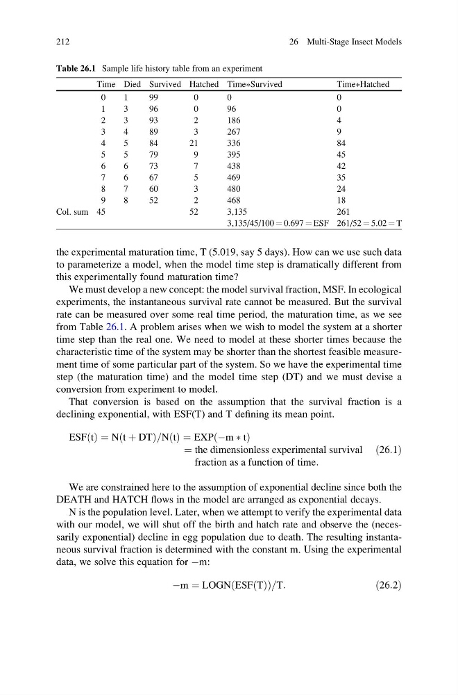
rate can be measured over some real time period, the maturation time, as we see
from Table 26.1. A problem arises when we wish to model the system at a shorter
time step than the real one. We need to model at these shorter times because the
characteristic time of the system may be shorter than the shortest feasible measurement time of some particular part of the system. So we have the experimental time
step (the maturation time) and the model time step (DT) and we must devise a
conversion from experiment to model.
That conversion is based on the assumption that the survival fraction is a
declining exponential, with ESF(T) and T defining its mean point.
ESF t
ð Þ ¼ N t þ DT
ð
Þ=N t
ð Þ ¼ EXP Àm à t
ð
Þ
¼ the dimensionless experimental survival
fraction as a function of time:
ð26:1Þ
We are constrained here to the assumption of exponential decline since both the
DEATH and HATCH flows in the model are arranged as exponential decays.
N is the population level. Later, when we attempt to verify the experimental data
with our model, we will shut off the birth and hatch rate and observe the (necessarily exponential) decline in egg population due to death. The resulting instantaneous survival fraction is determined with the constant m. Using the experimental
data, we solve this equation for Àm:
Àm ¼ LOGN ESF T
ð Þ
ð
Þ =T:
ð26:2Þ
Table 26.1 Sample life history table from an experiment
Time Died Survived Hatched Time * Survived
Time * Hatched
0
1
99
0
0
0
1
3
96
0
96
0
2
3
93
2
186
4
3
4
89
3
267
9
4
5
84
21
336
84
5
5
79
9
395
45
6
6
73
7
438
42
7
6
67
5
469
35
8
7
60
3
480
24
9
8
52
2
468
18
Col. sum 45
52
3,135
261
3,135/45/100 ¼ 0.697 ¼ ESF 261/52 ¼ 5.02 ¼ T
212
26 Multi-Stage Insect Models
to parameterize a model, when the model time step is dramatically different from
this experimentally found maturation time?
We must develop a new concept: the model survival fraction, MSF. In ecological
experiments, the instantaneous survival rate cannot be measured. But the survival
rate can be measured over some real time period, the maturation time, as we see
from Table 26.1. A problem arises when we wish to model the system at a shorter
time step than the real one. We need to model at these shorter times because the
characteristic time of the system may be shorter than the shortest feasible measurement time of some particular part of the system. So we have the experimental time
step (the maturation time) and the model time step (DT) and we must devise a
conversion from experiment to model.
That conversion is based on the assumption that the survival fraction is a
declining exponential, with ESF(T) and T defining its mean point.
ESF t
ð Þ ¼ N t þ DT
ð
Þ=N t
ð Þ ¼ EXP Àm à t
ð
Þ
¼ the dimensionless experimental survival
fraction as a function of time:
ð26:1Þ
We are constrained here to the assumption of exponential decline since both the
DEATH and HATCH flows in the model are arranged as exponential decays.
N is the population level. Later, when we attempt to verify the experimental data
with our model, we will shut off the birth and hatch rate and observe the (necessarily exponential) decline in egg population due to death. The resulting instantaneous survival fraction is determined with the constant m. Using the experimental
data, we solve this equation for Àm:
Àm ¼ LOGN ESF T
ð Þ
ð
Þ =T:
ð26:2Þ
Table 26.1 Sample life history table from an experiment
Time Died Survived Hatched Time * Survived
Time * Hatched
0
1
99
0
0
0
1
3
96
0
96
0
2
3
93
2
186
4
3
4
89
3
267
9
4
5
84
21
336
84
5
5
79
9
395
45
6
6
73
7
438
42
7
6
67
5
469
35
8
7
60
3
480
24
9
8
52
2
468
18
Col. sum 45
52
3,135
261
3,135/45/100 ¼ 0.697 ¼ ESF 261/52 ¼ 5.02 ¼ T
212
26 Multi-Stage Insect Models