

this simplified approach seem to agree with those in the more elaborate model of
Starfield and Blelock, reconfirming our earlier statements that you should start with
simple models. These are often the most powerful ones.
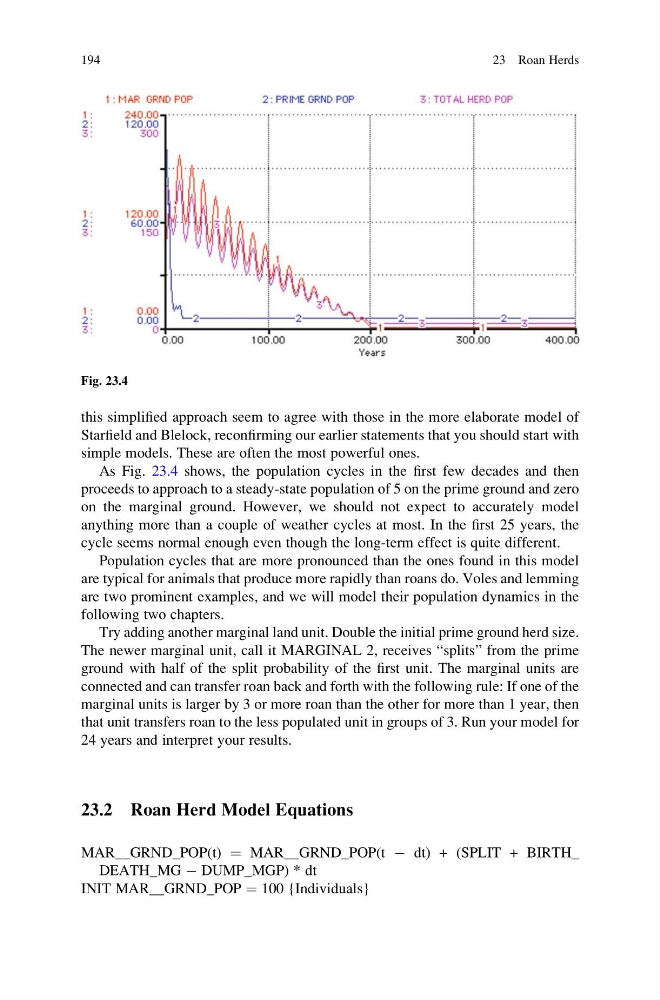
As Fig. 23.4 shows, the population cycles in the first few decades and then
proceeds to approach to a steady-state population of 5 on the prime ground and zero
on the marginal ground. However, we should not expect to accurately model
anything more than a couple of weather cycles at most. In the first 25 years, the
cycle seems normal enough even though the long-term effect is quite different.
Population cycles that are more pronounced than the ones found in this model
are typical for animals that produce more rapidly than roans do. Voles and lemming
are two prominent examples, and we will model their population dynamics in the
following two chapters.
Try adding another marginal land unit. Double the initial prime ground herd size.
The newer marginal unit, call it MARGINAL 2, receives “splits” from the prime
ground with half of the split probability of the first unit. The marginal units are
connected and can transfer roan back and forth with the following rule: If one of the
marginal units is larger by 3 or more roan than the other for more than 1 year, then
that unit transfers roan to the less populated unit in groups of 3. Run your model for
24 years and interpret your results.
23.2 Roan Herd Model Equations
MAR__GRND_POP(t) ¼ MAR__GRND_POP(t À dt) + (SPLIT + BIRTH_
DEATH_MG À DUMP_MGP) * dt
INIT MAR__GRND_POP ¼ 100 {Individuals}
Fig. 23.4
194
23 Roan Herds
Starfield and Blelock, reconfirming our earlier statements that you should start with
simple models. These are often the most powerful ones.
As Fig. 23.4 shows, the population cycles in the first few decades and then
proceeds to approach to a steady-state population of 5 on the prime ground and zero
on the marginal ground. However, we should not expect to accurately model
anything more than a couple of weather cycles at most. In the first 25 years, the
cycle seems normal enough even though the long-term effect is quite different.
Population cycles that are more pronounced than the ones found in this model
are typical for animals that produce more rapidly than roans do. Voles and lemming
are two prominent examples, and we will model their population dynamics in the
following two chapters.
Try adding another marginal land unit. Double the initial prime ground herd size.
The newer marginal unit, call it MARGINAL 2, receives “splits” from the prime
ground with half of the split probability of the first unit. The marginal units are
connected and can transfer roan back and forth with the following rule: If one of the
marginal units is larger by 3 or more roan than the other for more than 1 year, then
that unit transfers roan to the less populated unit in groups of 3. Run your model for
24 years and interpret your results.
23.2 Roan Herd Model Equations
MAR__GRND_POP(t) ¼ MAR__GRND_POP(t À dt) + (SPLIT + BIRTH_
DEATH_MG À DUMP_MGP) * dt
INIT MAR__GRND_POP ¼ 100 {Individuals}
Fig. 23.4
194
23 Roan Herds