

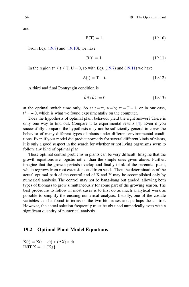
and
B T
ð Þ ¼ 1:
ð19:10Þ
From Eqs. (19.8) and (19.10), we have
B t
ð Þ ¼ 1:
ð19:11Þ
In the region t* t T, U ¼ 0, so with Eqs. (19.7) and (19.11) we have
A t
ð Þ ¼ T À t:
ð19:12Þ
A third and final Pontryagin condition is
∂H=∂U ¼ 0
ð19:13Þ
at the optimal switch time only. So at t ¼ t*, a ¼ b; t* ¼ T À 1, or in our case,
t* ¼ 4.0, which is what we found experimentally on the computer.
Does the hypothesis of optimal plant behavior yield the right answer? There is
only one way to find out. Compare it to experimental results [4]. Even if you
successfully compare, the hypothesis may not be sufficiently general to cover the
behavior of many different types of plants under different environmental conditions. Even if your model did predict correctly for several different kinds of plants,
it is only a good suspect in the search for whether or not living organisms seem to
follow any kind of optimal plan.
These optimal control problems in plants can be very difficult. Imagine that the
growth equations are logistic rather than the simple ones given above. Further,
imagine that the growth periods overlap and finally think of the perennial plant,
which regrows from root extensions and from seeds. Then the determination of the
actual optimal path of the control and of X and Y may be accomplished only by
numerical analysis. The control may not be bang-bang but graded, allowing both
types of biomass to grow simultaneously for some part of the growing season. The
best procedure to follow in most cases is to first do as much analytical work as
possible to simplify the ensuing numerical analysis. Usually, one of the costate
variables can be found in terms of the two biomasses and perhaps the control.
However, the actual solution frequently must be obtained numerically even with a
significant quantity of numerical analysis.
19.2 Optimal Plant Model Equations
X(t) ¼ X(t À dt) + (ΔX) * dt
INIT X ¼ .1 {Kg}
154
19 The Optimum Plant
B T
ð Þ ¼ 1:
ð19:10Þ
From Eqs. (19.8) and (19.10), we have
B t
ð Þ ¼ 1:
ð19:11Þ
In the region t* t T, U ¼ 0, so with Eqs. (19.7) and (19.11) we have
A t
ð Þ ¼ T À t:
ð19:12Þ
A third and final Pontryagin condition is
∂H=∂U ¼ 0
ð19:13Þ
at the optimal switch time only. So at t ¼ t*, a ¼ b; t* ¼ T À 1, or in our case,
t* ¼ 4.0, which is what we found experimentally on the computer.
Does the hypothesis of optimal plant behavior yield the right answer? There is
only one way to find out. Compare it to experimental results [4]. Even if you
successfully compare, the hypothesis may not be sufficiently general to cover the
behavior of many different types of plants under different environmental conditions. Even if your model did predict correctly for several different kinds of plants,
it is only a good suspect in the search for whether or not living organisms seem to
follow any kind of optimal plan.
These optimal control problems in plants can be very difficult. Imagine that the
growth equations are logistic rather than the simple ones given above. Further,
imagine that the growth periods overlap and finally think of the perennial plant,
which regrows from root extensions and from seeds. Then the determination of the
actual optimal path of the control and of X and Y may be accomplished only by
numerical analysis. The control may not be bang-bang but graded, allowing both
types of biomass to grow simultaneously for some part of the growing season. The
best procedure to follow in most cases is to first do as much analytical work as
possible to simplify the ensuing numerical analysis. Usually, one of the costate
variables can be found in terms of the two biomasses and perhaps the control.
However, the actual solution frequently must be obtained numerically even with a
significant quantity of numerical analysis.
19.2 Optimal Plant Model Equations
X(t) ¼ X(t À dt) + (ΔX) * dt
INIT X ¼ .1 {Kg}
154
19 The Optimum Plant